

Table 1
Summary of existing empirical panel fiscal sustainability test
| Reference | Sustainability test | Period and country | Findings |
|---|---|---|---|
| Afonso and Rault (2010) | Stationarity of debt and cointegration between revenue and expenditure | 15 Selected EU countries (1970–2006) | Fiscal stance sustainability confirmed |
| Baldi and Staehr (2015) | Estimated fiscal reaction function of primary balance, debt and business cycle viables | Different groups of EU countries (2001–2004) | Sustainable fiscal stance for all groups post financial crises |
| Beqiraj et al. (2018) | Panel cointegration test between primary balance and public debt | 21 OECD countries (1991–2015) | Fiscal stance judged to be unsustainable |
| Boekemeier and Stoian (2018) | Fiscal reaction function of primary balance and debt | CEEC (1997–2013) | Fiscal stance sustainable for selected countries |
| Brady and Magazzino (2018) | Stationarity of public debt | 19 European countries (1970–2016) | Fiscal stance sustainability confirmed |
| Checherita-Wesphal and Žďárek (2017) | Fiscal reaction function of primary balance response to debt | 18 Euro Area countries (1970–2013) | Sustainable fiscal stance |
| Claeys (2007) | Cointegration between revenue, spending and net interest payment | Selected European countries (1970–2001) | Sustainable fiscal policy |
| Krajewski et al. (2016) | Cointegration between revenue and expenditure and a fiscal reaction function | CEEC (1990–2012) | Sustainable fiscal stance |
| Lee et al. (2018) | Fiscal reaction function of primary balance response to debt | EU regional groups (1950–2014) | Varied results depending on the region |
| Llorca and Redzepagic (2008) | Cointegration between revenue and expenditure | CEEC (1999:1–2006:1) | Fiscal stance sustainable in selected countries |
| Prohl and Schneider (2006) | Cointegration between budget deficit and public debt | 15 EU countries (1970–2004) | Fiscal stance sustainability confirmed |
| Westerlund and Prohl (2010) | Cointegration between revenue and expenditure | 8 rich OECD countries (1977:1–2006:4) | Sustainability hypothesis confirmed for selected countries |
[i] CEEC, Central and Eastern European Countries; EU, European Union; OECD, Organisation for Economic Corporation and Development.
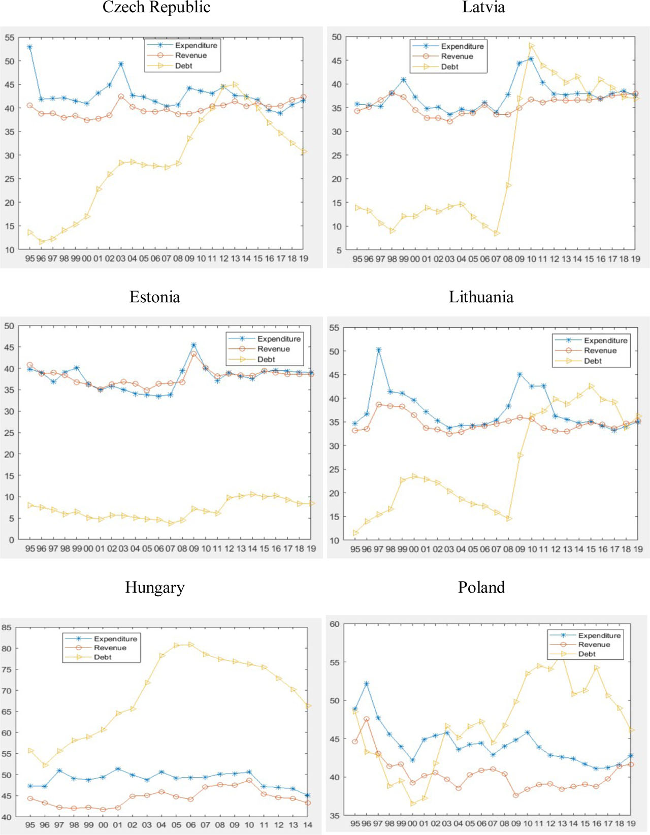
Figure 1
Revenue, Expenditure, and public debt
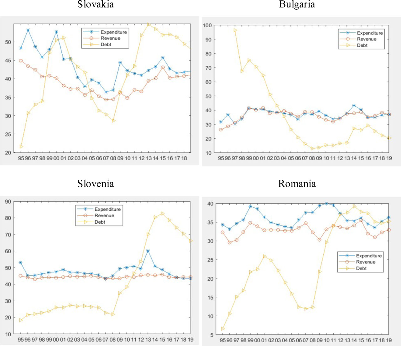
Figure 2
Revenue, Expenditure, and public debt
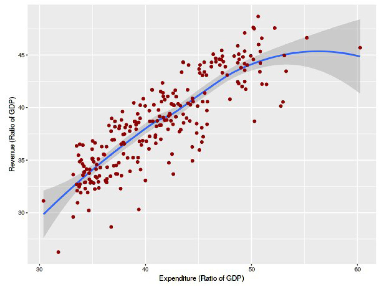
Figure 3
Panel scatter plot
Table 2
Dates of structural breaks for individual series
| Countries (CEEC) | Revenue | Expenditure |
|---|---|---|
| Czechia | 2002, 2010 | 2003 |
| Estonia | 1998, 2008, 2011 | 1999, 2007, 2010 |
| Hungary | 1997, 2006, 2011, 2015 | 1998, 2001, 2015 |
| Latvia | 1999, 2009 | 1997, 2000, 2008, 2011 |
| Lithuania | 2000 | 2000, 2008, 2011 |
| Poland | 1997, 2008, 2015 | 1997, 2011 |
| Slovakia | 1997, 2000, 2003, 2012 | 2002, 2008 |
| Slovenia | 2011, 2015 | 2008, 2015 |
| Bulgaria | 1997, 2008, 2012 | 1998, 2002 |
| Romania | 1997 | 1998, 2001, 2006, 2012 |
[i] CEEC, Central and Eastern European Countries.
Table 3
Panel summary Statistics
| Revenue-GDP ratio | Expenditure-GDP ratio | Debt-GDP ratio | |
|---|---|---|---|
| Mean | 0.391 | 0.419 | 0.340 |
| Standard Deviation | 0.039 | 0.505 | 0.178 |
| Maximum | 0.482 | 0.541 | 0.711 |
| Minimum | 0.308 | 0.321 | 0.038 |
| Observations | 250 | 250 | 250 |
Table 4
Deficit to GDP ratio
| Year | Czh | Est | Hun | Lat | Lith | Pol | Svk | Slvn | Bulg | Rom |
|---|---|---|---|---|---|---|---|---|---|---|
| 1995 | −12.44 | 1.05 | −8.60 | −1.43 | −1.53 | −4.26 | −3.47 | −8.15 | −5.52 | −2.00 |
| 1996 | −3.01 | −0.32 | −4.38 | −0.42 | −3.22 | −4.63 | −9.82 | −1.09 | −8.11 | −3.57 |
| 1997 | −3.19 | 2.15 | −5.55 | 1.42 | −11.59 | −4.61 | −6.27 | −2.31 | 0.76 | −4.43 |
| 1998 | −4.19 | −0.73 | −7.39 | 0.03 | −3.03 | −4.21 | −5.30 | −2.33 | 1.08 | −3.24 |
| 1999 | −3.14 | −3.29 | −5.23 | −3.74 | −2.82 | −2.28 | −7.17 | −2.97 | 0.09 | −4.42 |
| 2000 | −3.57 | −0.04 | −2.980 | −2.73 | −3.17 | −2.98 | −12.63 | −3.65 | −0.53 | −4.60 |
| 2001 | −5.48 | 0.20 | −3.94 | −1.95 | −3.51 | −4.77 | −7.22 | −4.45 | 1.05 | −3.46 |
| 2002 | −6.36 | 0.42 | −8.76 | −2.29 | −1.85 | −4.85 | −8.22 | −2.37 | −1.16 | −1.93 |
| 2003 | −6.89 | 1.82 | −7.11 | −1.46 | −1.27 | −6.08 | −3.12 | −2.56 | −0.39 | −1.43 |
| 2004 | −2.39 | 2.34 | −6.52 | −0.92 | −1.39 | −5.04 | −2.32 | −1.94 | 1.80 | −1.09 |
| 2005 | −2.9 | 1.08 | −7.72 | −0.36 | −0.34 | −3.96 | −2.87 | −1.32 | 1.00 | −0.81 |
| 2006 | −2.17 | 2.87 | −9.21 | −0.49 | −0.27 | −3.56 | −3.58 | −1.23 | 1.81 | −2.14 |
| 2007 | −0.65 | 2.73 | −5.03 | −0.51 | −0.81 | −1.85 | −2.05 | −0.05 | 1.10 | −2.73 |
| 2008 | −1.98 | −2.65 | −3.73 | −4.20 | −3.09 | −3.60 | −2.52 | −1.39 | 1.59 | −5.35 |
| 2009 | −5.45 | −2.16 | −4.69 | −9.49 | −9.13 | −7.25 | −8.15 | −5.81 | −4.05 | −9.06 |
| 2010 | −4.19 | 0.19 | −4.39 | −8.60 | −6.92 | −7.40 | −7.46 | −5.60 | −3.13 | −6.92 |
| 2011 | −2.73 | 1.06 | −5.19 | −4.25 | −8.95 | −4.88 | −4.46 | −6.63 | −1.98 | −5.43 |
| 2012 | −3.93 | −0.29 | −2.27 | −1.22 | −3.15 | −3.74 | −4.37 | −4.0 | −0.32 | −3.65 |
| 2013 | −1.25 | 0.18 | −2.54 | −1.17 | −2.61 | −4.18 | −2.87 | −14.58 | −0.43 | −2.10 |
| 2014 | −2.10 | 0.70 | −2.76 | −1.44 | −0.62 | −3.65 | −3.11 | −5.51 | −5.43 | −1.19 |
| 2015 | −0.61 | 0.14 | −1.97 | −1.36 | −0.27 | −2.62 | −2.67 | −2.85 | −1.72 | −0.61 |
| 2016 | 0.72 | −0.52 | −1.76 | 0.06 | 0.23 | −2.37 | −2.48 | −1.94 | 0.09 | −2.62 |
| 2017 | 1.56 | −0.77 | −2.38 | −0.52 | 0.45 | −1.46 | −0.95 | −0.01 | 1.10 | −2.64 |
| 2018 | 1.09 | −0.56 | −2.29 | −0.74 | 0.60 | −0.24 | −1.06 | 0.77 | 1.75 | −2.96 |
| 2019 | 0.75 | −0.30 | −1.83 | 0.51 | 0.13 | −1.16 | −1.03 | 0.72 | −0.11 | −3.33 |
[i] Highlights in bold indicates violation of the EU SGP.
[ii] Source: Author's own computations.
[iii] EU, European Union; SGP, Stability and Growth Pact.
Table 5
Breusch–Pagan and Pesaran cross-sectional dependence test
| Variables | Breusch–Pagan CD test | Pesaran CD test |
|---|---|---|
| Chi-square, P-value | z-value, P-value | |
| Expenditure to GDP ratio | 107.84, 0.000 | 5.494, 0.000 |
| Revenue to GDP ratio | 113.42, 0.000 | 1.716, 0.0862 |
[i] Pooled group variable by country. Null hypothesis of the test implies cross-sectional independence for both Breusch–Pagan and Pesaran test.
[ii] CD, cross-sectional dependence.
Table 6
Chow test of poolability of coefficients (5% significance level)
| Restricted model | Intercept | F-statistics | P-value | Verdict |
|---|---|---|---|---|
| FE (within) | Variable | 2.8438 | 0.004 | Not poolable |
| Pooled OLS | Fixed | 14.892 | 0.000 | Not poolable |
[i] Null hypothesis implies ‘model stability’ or constant coefficient.
[ii] FE, fixed effect; OLS, ordinary least square estimator.
Table 7
Panel stationarity test – Expenditure
| Countries | Constant | Constant and trend | ||||
|---|---|---|---|---|---|---|
| k = 1 | k = 2 | k = 3 | k = 1 | k = 2 | k = 3 | |
| Czechia | 0.070 | 0.309 | 0.302 | 0.050* | 0.059 | 0.050 |
| Estonia | 0.099 | 0.410* | 0.331 | 0.052* | 0.124* | 0.125* |
| Hungary. | 0.203** | 0.298 | 0.201 | 0.044 | 0.101 | 0.091 |
| Latvia | 0.183** | 0.504** | 0.414* | 0.051* | 0.080 | 0.083 |
| Lithuania | 0.052 | 0.055 | 0.116 | 0.051* | 0.043 | 0.051 |
| Poland | 0.182** | 0.496* | 0.416* | 0.053* | 0.056 | 0.076 |
| Slovakia | 0.048 | 0.219 | 0.197 | 0.040 | 0.145** | 0.139* |
| Slovenia | 0.059 | 0.189 | 0.322 | 0.054* | 0.097 | 0.085 |
| Bulgaria | 0.148** | 0.089 | 0.095 | 0.051* | 0.088 | 0.087 |
| Romania | 0.124 | 0.313 | 0.181 | 0.053* | 0.136** | 0.133* |
| Panel statistic | 2.995*** | 3.508*** | 2.282*** | 4.938*** | 3.309*** | 2.460*** |
| (0.001) | (0.000) | (0.011) | (0.000) | (0.000) | (0.007) | |
[i] Fourier panel stationarity test for 10 CEEC under the Null hypothesis of stationarity. P-values are for one sided test based on normal distribution.
[ii] Critical values (obtained from Becker et al. 2006, p. 289) for individual test statistics are as follows: 0.1318 (10%), 0.1720 (5%), 0.2699 (1%) for k = 1; 0.3150 (10%), 0.4152 (5%), 0.6671 (1%) for k = 2; 0.3393 (10%), 0.4480 (5%), 0.7182 (1%) for k = 3.
[iii] Critical values for constant and trend are as follows: 0.0471 (10%), 0.0546 (5%), 0.0716 (1%) for k = 1; 0.1034 (10%), 0.1321 (5%), 0.2022 (1%) for k = 2; 0.1141 (10%), 0.1423 (5%), 0.2103 (1%) for k = 3.
[v] CEEC, Central and Eastern European Countries.
Table 8
Panel stationarity test – Revenue
| Countries | Constant | Constant and trend | ||||
|---|---|---|---|---|---|---|
| k = 1 | k = 2 | k = 3 | k = 1 | k = 2 | k = 3 | |
| Czechia | 0.146* | 0.314 | 0.408* | 0.047 | 0.048 | 0.068 |
| Estonia | 0.157* | 0.271 | 0.108 | 0.044 | 0.066 | 0.091 |
| Hungary. | 0.342*** | 0.187 | 0.148 | 0.040 | 0.107* | 0.103 |
| Latvia | 0.070 | 0.448** | 0.313 | 0.052* | 0.074 | 0.076 |
| Lithuania | 0.074 | 0.155 | 0.299 | 0.051* | 0.076 | 0.054 |
| Poland | 0.170* | 0.409* | 0.352* | 0.065** | 0.101 | 0.103 |
| Slovakia | 0.262** | 0.371* | 0.362* | 0.057** | 0.153** | 0.143** |
| Slovenia | 0.056 | 0.128 | 0.239 | 0.056* | 0.079 | 0.074 |
| Bulgaria | 0.268** | 0.115 | 0.121 | 0.065** | 0.114* | 0.102 |
| Romania | 0.074 | 0.151 | 0.160 | 0.049* | 0.121* | 0.116* |
| Panel statistic | 5.652*** | 2.716*** | 2.136*** | 5.606*** | 3.405*** | 2.523*** |
| (0.000) | (0.003) | (0.016) | (0.000) | (0.000) | (0.006) | |
[i] Fourier panel stationarity test for 10 CEEC under the Null hypothesis of stationarity. P-values are for one sided test based on normal distribution.
[ii] Critical values (obtained from Becker et al. 2006, p. 289) for individual test statistics are as follows: 0.1318 (10%), 0.1720 (5%), 0.2699 (1%) for k = 1; 0.3150 (10%), 0.4152 (5%), 0.6671 (1%) for k = 2; 0.3393 (10%), 0.4480 (5%), 0.7182 (1%) for k = 3.
[iii] Critical values for constant and trend are as follows: 0.0471 (10%), 0.0546 (5%), 0.0716 (1%) for k = 1; 0.1034 (10%), 0.1321 (5%), 0.2022 (1%) for k = 2; 0.1141 (10%), 0.1423 (5%), 0.2103 (1%) for k = 3.
[v] CEEC, Central and Eastern European Countries.
Table 9
Panel cointegration test of revenue and expenditure – Europe
| Zτ (N) | Zφ(N) | |||
|---|---|---|---|---|
| Models | Value (τ) | P-value | Value (φ) | P-value |
| No breaks | −1.515 | 0.065 | −0.963 | 0.168 |
| Level break | 0.879 | 0.810 | 0.690 | 0.755 |
| Regime shift | 0.422 | 0.663 | 0.437 | 0.669 |
| Number of observations | 250 | 250 | ||
[i] Westerlund and Edgerton (2008) cointegration test with three maximum number of breaks in the cointegration relationship, which are determined by grid search at the minimum of the SSR. Null hypothesis indicates ‘No cointegration’. Displayed P-values are based on one-sided normal distribution test. *, ** and *** denote rejection of the null hypothesis at 10%, 5% and 1% respectively.
[ii] SSR, sum of squared residuals.
Table 10
Panel Cointegration cointegration test of cyclically adjusted revenue and cyclically adjusted spending
| Zτ(N) | Zφ(N) | |||
|---|---|---|---|---|
| Models | Value (τ) | P-value | Value (φ) | P-value |
| No breaks | −2.842*** | 0.002 | −3.587*** | 0.000 |
| Level break | −3.076*** | 0.001 | −2.950*** | 0.002 |
| Regime shift | −2.368*** | 0.009 | −2.984*** | 0.001 |
| Number of observations | 220 | 220 | ||
[i] Westerlund and Edgerton (2008) cointegration test with three maximum number of breaks in the cointegration relationship which are determined by grid search at the minimum of the SSR. Null hypothesis indicates ‘No cointegration’. Displayed P-values are based on one-sided normal distribution test.
[iii] Hamiliton Filter is used to obtain cyclically adjusted revenues and expenditures.
[iv] SSR, sum of squared residuals.
Table 11
Long run coefficient for cyclically adjusted fiscal variables
| Stat | MG | CCEMG | MG-FMOLS | MG-DOLSa |
|---|---|---|---|---|
| γ | 0.499 | 0.364 | 0.938 | 0.935 |
| Test stat | 3.390 | 3.815 | 480.74 | 604.07 |
| P-value | 0.000 | 0.000 | 0.000 | 0.000 |
| Std error | 0.147 | 0.095 | 0.002 | 0.02 |
| Obs | 220 | 220 | 210 | 130 |
| Shapiro–Wilk Normality test | 0.970 | 0.977 | 0.992 | 0.986 |
| P-value | (0.000) | (0.001) | (0.260) | (0.220) |
| Peseran CD test | 3.652 | −2.411 | 3.328 | −0.260 |
| P-value | (0.000) | (0.016) | (0.001) | (0.795) |
a Reported lags and leads of 4 for MG-DOLS. The study explored lags and leads from 1 to 4; however, this does not change the estimates of the parameter.
CCEMG, common correlated effect mean group; CD, cross-sectional dependence; DOLS, dyanmic OLS; FMOLS, fully modified OLS; MG, mean group; OLS, ordinary least square estimator.
Table 12
Wald test of coefficient and confidence intervals
Table A1
Panel stationarity test – first difference of expenditure
| Countries | Constant | Constant and trend | ||||
|---|---|---|---|---|---|---|
| k = 1 | k = 2 | k = 3 | k = 1 | k = 2 | k = 3 | |
| Czechia | 0.195** | 0.170 | 0.132 | 0.059** | 0.094 | 0.093 |
| Estonia | 0.032 | 0.033 | 0.065 | 0.031 | 0.035 | 0.031 |
| Hungary. | 0.078 | 0.091 | 0.110 | 0.048* | 0.089 | 0.107 |
| Latvia | 0.057 | 0.126 | 0.070 | 0.046 | 0.050 | 0.046 |
| Lithuania | 0.078 | 0.148 | 0.080 | 0.053* | 0.097 | 0.060 |
| Poland | 0.075 | 0.044 | 0.055 | 0.045 | 0.038 | 0.051 |
| Slovakia | 0.122 | 0.136 | 0.137 | 0.047 | 0.083 | 0.088 |
| Slovenia | 0.064 | 0.131 | 0.097 | 0.060** | 0.111* | 0.096 |
| Bulgaria | 0.069 | 0.114 | 0.123 | 0.031 | 0.091 | 0.096 |
| Romania | 0.053 | 0.069 | 0.181 | 0.052* | 0.040 | 0.068 |
| Panel statistic | 0.970 | −0.827 | −1.336 | 4.437*** | 1.674** | 1.034 |
| (0.166) | (0.796) | (0.909) | (0.000) | (0.047) | (0.151) | |
[i] Fourier panel stationarity test for 10 CEEC under the Null hypothesis of stationarity.
[ii] Critical values (obtained from Becker et al., 2006, p. 289) for individual test statistics are as follows: 0.1318 (10%), 0.1720 (5%), 0.2699 (1%) for k = 1; 0.3150 (10%), 0.4152 (5%), 0.6671 (1%) for k = 2; 0.3393 (10%), 0.4480 (5%), 0.7182 (1%) for k = 3.
[iii] Critical values for constant and trend are as follows: 0.0471 (10%), 0.0546 (5%), 0.0716 (1%) for k = 1; 0.1034 (10%), 0.1321 (5%), 0.2022 (1%) for k = 2; 0.1141 (10%), 0.1423 (5%), 0.2103 (1%) for k = 3.
[v] CEEC, Central and Eastern European Countries.
Table A2
Panel stationarity Test test -– First first difference of Revenuerevenue
| Countrs | Constant | Constant and trend | ||||
|---|---|---|---|---|---|---|
| k = 1 | k = 2 | k = 3 | k = 1 | k = 2 | k = 3 | |
| Czechia | 0.127 | 0.075 | 0.074 | 0.044 | 0.057 | 0.074 |
| Estonia | 0.093 | 0.082 | 0.117 | 0.051* | 0.071 | 0.111 |
| Hungary. | 0.038 | 0.151 | 0.159 | 0.031 | 0.148** | 0.153** |
| Latvia | 0.063 | 0.062 | 0.107 | 0.047 | 0.052 | 0.056 |
| Lithuania | 0.081 | 0.122 | 0.079 | 0.061** | 0.082 | 0.077 |
| Poland | 0.088 | 0.128 | 0.157 | 0.057** | 0.056 | 0.060 |
| Slovakia | 0.108 | 0.531** | 0.423* | 0.076*** | 0.120* | 0.099 |
| Slovenia | 0.061 | 0.108 | 0.117 | 0.057** | 0.101 | 0.077 |
| Bulgaria | 0.180** | 0.327 | 0.366* | 0.027 | 0.149** | 0.159** |
| Romania | 0.038 | 0.065 | 0.083 | 0.035 | 0.048 | 0.041 |
| Panel statistic | 1.282 | 0.574 | 0.292 | 4.723*** | 2.965*** | 2.357*** |
| (0.100) | (0.283) | (0.385) | (0.000) | (0.002) | (0.009) | |
[i] Fourier panel stationarity test for 10 CEEC under the Null hypothesis of stationarity.
[ii] Critical values (obtained from Becker et al., 2006, p. 289) for individual test statistics are as follows: 0.1318 (10%), 0.1720 (5%), 0.2699 (1%) for k = 1; 0.3150 (10%), 0.4152 (5%), 0.6671 (1%) for k = 2; 0.3393 (10%), 0.4480 (5%), 0.7182 (1%) for k = 3.
[iii] Critical values for constant and trend are as follows: 0.0471 (10%), 0.0546 (5%), 0.0716 (1%) for k = 1; 0.1034 (10%), 0.1321 (5%), 0.2022 (1%) for k = 2; 0.1141 (10%), 0.1423 (5%), 0.2103 (1%) for k = 3.
[v] CEEC, Central and Eastern European Countries.
Table A3
Panel Stationarity stationarity test with sharp breaks - – Robustness robustness check
| Panel - – Panel test (revenue) | ||
| Model | Level | First difference |
| Break (Homogeneous) | 1.762 (0.039)** | 0.426 (0.335) |
| Breaks (Heterogeneous) | 2.975 (0.001)*** | 0.152 (0.440) |
| Panel B – Panel stationarity test (expenditure) | ||
| Model | Level | First difference |
| Break (Homogeneous) | 1.687 (0.046)** | 0.137 (0.446) |
| Breaks (Heterogeneous) | 2.031 (0.021)** | 0.630 (0.264) |
[i] Panel test by Carrion-i-Silvestre et al. (2005). Reported test statistics and P-values in parenthesis.
Table A4
Panel stationarity test – cyclically adjusted expenditure
| Countries | Constant | Constant and trend | ||||
|---|---|---|---|---|---|---|
| k = 1 | k = 2 | k = 3 | k = 1 | k = 2 | k = 3 | |
| Czechia | 0.144* | 0.165 | 0.132 | 0.065** | 0.134** | 0.126** |
| Estonia | 0.080 | 0.401 | 0.385* | 0.046 | 0.105* | 0.092 |
| Hungary. | 0.157* | 0.096 | 0.068 | 0.059** | 0.100 | 0.126** |
| Latvia | 0.106 | 0.202 | 0.155 | 0.045 | 0.080 | 0.073 |
| Lithuania | 0.089 | 0.172 | 0.146 | 0.072*** | 0.135** | 0.126** |
| Poland | 0.154* | 0.466** | 0.577** | 0.047 | 0.074 | 0.073 |
| Slovakia | 0.095 | 0.258 | 0.206 | 0.063** | 0.146** | 0.126** |
| Slovenia | 0.091 | 0.488** | 0.332 | 0.070** | 0.140** | 0.093 |
| Bulgaria | 0.102 | 0.072 | 0.097 | 0.068** | 0.072 | 0.065 |
| Romania | 0.064 | 0.087 | 0.110 | 0.049* | 0.089 | 0.110 |
| Panel statistic | 2.491*** | 2.376*** | 1.461* | 7.017*** | 4.511*** | 2.885*** |
| (0.006) | (0.009) | (0.072) | (0.000) | (0.000) | (0.002) | |
[i] Fourier panel stationarity test for 10 CEEC under the Null hypothesis of stationarity.
[ii] Critical values (obtained from Becker et al., 2006, p. 289) for individual test statistics are as follows: 0.1318 (10%), 0.1720 (5%), 0.2699 (1%) for k = 1; 0.3150 (10%), 0.4152 (5%), 0.6671 (1%) for k = 2; 0.3393 (10%), 0.4480 (5%), 0.7182 (1%) for k = 3.
[iii] Critical values for constant and trend are as follows 0.0471 (10%), 0.0546 (5%), 0.0716 (1%) for k = 1; 0.1034 (10%), 0.1321 (5%), 0.2022 (1%) for k = 2; 0.1141 (10%), 0.1423 (5%), 0.2103 (1%) for k = 3
[v] CEEC, Central and Eastern European Countries.
Table A5
Panel stationarity Test test -– Cyclically cyclically adjusted revenue
| Countrs | Constant | Constant and trend | ||||
|---|---|---|---|---|---|---|
| k = 1 | k = 2 | k = 3 | k = 1 | k = 2 | k = 3 | |
| Czechia | 0.160* | 0.416** | 0.519** | 0.048* | 0.070 | 0.060 |
| Estonia | 0.079 | 0.414* | 0.249 | 0.044 | 0.042 | 0.089 |
| Hungary | 0.040 | 0.398* | 0.348* | 0.039 | 0.058 | 0.103 |
| Latvia | 0.037 | 0.324* | 0.356* | 0.037 | 0.036 | 0.051 |
| Lithuania | 0.061 | 0.242 | 0.165 | 0.059** | 0.145** | 0.111 |
| Poland | 0.241** | 0.434** | 0.435* | 0.078*** | 0.056 | 0.072 |
| Slovakia | 0.080 | 0.262 | 0.230 | 0.056** | 0.149** | 0.123* |
| Slovenia | 0.097 | 0.237 | 0.261 | 0.075*** | 0.132* | 0.066 |
| Bulgaria | 0.040 | 0.281 | 0.343* | 0.037 | 0.035 | 0.071 |
| Romania | 0.083 | 0.246 | 0.338 | 0.054* | 0.044 | 0.073 |
| Panel statistic | 1.524*** | 4.395*** | 3.768*** | 5.575*** | 1.985** | 1.682** |
| (0.064) | (0.000) | (0.000) | (0.000) | (0.023) | (0.046) | |
[i] Fourier panel stationarity test for 10 CEEC under the Null hypothesis of stationarity.
[ii] Critical values (obtained from Becker et al., 2006, p. 289) for individual test statistics are as follows: 0.1318 (10%), 0.1720 (5%), 0.2699 (1%) for k = 1; 0.3150 (10%), 0.4152 (5%), 0.6671 (1%) for k = 2; 0.3393 (10%), 0.4480 (5%), 0.7182 (1%) for k = 3.
[iii] Critical values for constant and trend are as follows 0.0471 (10%), 0.0546 (5%), 0.0716 (1%) for k = 1; 0.1034 (10%), 0.1321 (5%), 0.2022 (1%) for k = 2; 0.1141 (10%), 0.1423 (5%), 0.2103 (1%) for k = 3.
[v] CEEC, Central and Eastern European Countries.
Table A6
Panel stationarity test – first difference of cyclically adjusted expenditure
| Countries | Constant | Constant and trend | ||||
|---|---|---|---|---|---|---|
| k = 1 | k = 2 | k = 3 | k = 1 | k = 2 | k = 3 | |
| Czechia | 0.224** | 0.255 | 0.298 | 0.140*** | 0.142** | 0.137* |
| Estonia | 0.041 | 0.105 | 0.061 | 0.037 | 0.043 | 0.045 |
| Hungary. | 0.059 | 0.141 | 0.144 | 0.045 | 0.141** | 0.131* |
| Latvia | 0.076 | 0.075 | 0.068 | 0.056** | 0.063 | 0.068 |
| Lithuania | 0.121 | 0.211 | 0.194 | 0.119*** | 0.126* | 0.118* |
| Poland | 0.193* | 0.191 | 0.198 | 0.051* | 0.120* | 0.144** |
| Slovakia | 0.044 | 0.304 | 0.204 | 0.036 | 0.036 | 0.063 |
| Slovenia | 0.138* | 0.189 | 0.147 | 0.108*** | 0.137** | 0.074 |
| Bulgaria | 0.102 | 0.073 | 0.142 | 0.049* | 0.051 | 0.061 |
| Romania | 0.042 | 0.147 | 0.055 | 0.038 | 0.048 | 0.044 |
| Panel statistic | 2.237** | 0.668 | −0.086 | 9.258*** | 3.130*** | 2.196** |
| (0.013) | (0.252) | (0.532) | (0.000) | (0.001) | (0.014) | |
[i] Fourier panel stationarity test for 10 CEEC under the Null hypothesis of stationarity.
[ii] Critical values (obtained from Becker et al., 2006, p. 289) for individual test statistics are as follows: 0.1318 (10%), 0.1720 (5%), 0.2699 (1%) for k = 1; 0.3150 (10%), 0.4152 (5%), 0.6671 (1%) for k = 2; 0.3393 (10%), 0.4480 (5%), 0.7182 (1%) for k = 3.
[iii] Critical values for constant and trend are as follows 0.0471 (10%), 0.0546 (5%), 0.0716 (1%) for k = 1; 0.1034 (10%), 0.1321 (5%), 0.2022 (1%) for k = 2; 0.1141 (10%), 0.1423 (5%), 0.2103 (1%) for k = 3.
[v] CEEC, Central and Eastern European Countries.
Table A7
Panel stationarity Test test -– First first difference of cyclically adjusted revenue
| Countrs | Constant | Constant and trend | ||||
|---|---|---|---|---|---|---|
| k = 1 | k = 2 | k = 3 | k = 1 | k = 2 | k = 3 | |
| Czechia | 0.060 | 0.092 | 0.168 | 0.058** | 0.068 | 0.067 |
| Estonia | 0.043 | 0.073 | 0.097 | 0.039 | 0.067 | 0.086 |
| Hungary. | 0.042 | 0.071 | 0.121 | 0.040 | 0.071 | 0.122* |
| Latvia | 0.093 | 0.096 | 0.092 | 0.093*** | 0.096 | 0.088 |
| Lithuania | 0.166* | 0.496** | 0.303 | 0.103*** | 0.130* | 0.104 |
| Poland | 0.217** | 0.187 | 0.286 | 0.033 | 0.071 | 0.089 |
| Slovakia | 0.102 | 0.244 | 0.214 | 0.102*** | 0.104* | 0.095 |
| Slovenia | 0.131 | 0.172 | 0.185 | 0.114*** | 0.197** | 0.088 |
| Bulgaria | 0.1068 | 0.085 | 0.117 | 0.063** | 0.077 | 0.116* |
| Romania | 0.120 | 0.071 | 0.052 | 0.039 | 0.047 | 0.042 |
| Panel statistic | 2.244** | 0.421 | 0.190 | 9.430*** | 3.306*** | 2.275** |
| (0.012) | (0.337) | (0.425) | (0.000) | (0.000) | (0.011) | |
[i] Fourier panel stationarity test for 10 CEEC under the Null hypothesis of stationarity.
[ii] Critical values (obtained from Becker et al., 2006, p. 289) for individual test statistics are as follows: 0.1318 (10%), 0.1720 (5%), 0.2699 (1%) for k = 1; 0.3150 (10%), 0.4152 (5%), 0.6671 (1%) for k = 2; 0.3393 (10%), 0.4480 (5%), 0.7182 (1%) for k = 3.
[iii] Critical values for constant and trend are as follows: 0.0471 (10%), 0.0546 (5%), 0.0716 (1%) for k = 1; 0.1034 (10%), 0.1321 (5%), 0.2022 (1%) for k = 2; 0.1141 (10%), 0.1423 (5%), 0.2103 (1%) for k = 3
[v] CEEC, Central and Eastern European Countries.
Table A8
Panel cointegration test of cyclically adjusted revenue and cyclically adjusted spending (HP Filter used for detrending series)
| Zτ(N) | Zφ(N) | |||
|---|---|---|---|---|
| Models | Value (τ) | P-value | Value (φ) | P-value |
| No breaks | 1.731 | 0.958 | −2.409*** | 0.008 |
| Level break | −1.984** | 0.024 | −2.490*** | 0.006 |
| Regime shift | −6.050*** | 0.000 | −7.182*** | 0.000 |
| Number of observations | 250 | 250 | ||
[i] Westerlund and Edgerton (2008) cointegration test. Maximum of three breaks are permitted. Displayed P-values are based on one-sided normal distribution test.
[iii] Maximum of three structural breaks in the cointegration relationship. Detrending of the series was done using the HP filter.
[iv] HP, Hodrick Prescott.