

Otaki and Tamai (2012) presented a microeconomic foundation of the negative relation between the unemployment rate and the inflation rate, that is, the Phillips Curve (Phillips, 1958) using an overlapping generations (OLG) model under monopolistic competition. They showed that, the lower the unemployment rate in a period (e.g., period t−1), the higher the inflation rate from period t to period t−1. Their logic is as follows. They assumed that the low (or high) unemployment rate in period t−1 increases (or decreases) the labour productivity in period t by learning effect. If the unemployment rate in period t−1 increases, the labour productivity in period t falls. Then, by the behaviour of firms in monopolistic competition, the price of the goods in period t rises given nominal wage rate, and the inflation rate from period t to period t+1 falls given the (expected) price of the goods in period t+1. Alternatively, a decrease in the unemployment rate in period t−1 increases the labour productivity in period t. Then, the price of the goods falls, and the inflation rate from period t to period t+1 increases given the (expected) price of the goods in period t+1. However, we do not find their conclusion that the low unemployment rate in period t−1 explains the high inflation rate from period t to period t+1 to be satisfactory. A fall in the price in period t means that the inflation rate from period t−1 to period t falls, that is, the low unemployment rate in period t−1 explains the low (not high) inflation rate from period t−1 to period t in their model.
Instead, in this article, we consider the effects of a change in the nominal wage rate with negative real balance effect. We use a three-period (three generations) OLG model with childhood period, younger period and older period. Also, we consider a pay-as-you-go pension system for the older generation to bring about negative real balance effect of a fall in the nominal wage rate. The negative real balance effect (or negative Pigou effect) means that by falls in the nominal wage rate and the price of the goods the real asset of consumers (difference between net savings and debts multiplied by marginal propensity to consume) decreases. The net savings of consumers is the difference between the consumption of consumers in Period 2 (when they are old) and pay-as-you-go pensions.
We will show the negative relationship between the unemployment rate and the inflation rate in the same period. Our logic is as follows. If the nominal wage rate in a period, for example, period t falls, the price of the goods falls. This means that the inflation rate from period t−1 to period t decreases. By the negative real balance effect, the aggregate demand for the goods and employment decreases and the unemployment rate increases in period t. Alternatively, if the nominal wage rate in period t rises, the price of the goods rises, and the inflation rate from period t−1 to period t increases. By the negative real balance effect, the aggregate demand for the goods and employment increases and the unemployment rate decreases in period t. For details, refer Section 4.
There are various studies on the theoretical basis of the Phillips curve from the neoclassical and new Keynesian standpoint. The representative of neoclassical studies is given (Lucas 1972). The neoclassical Phillips curve based on the rational expectation hypothesis is vertical at the natural unemployment rate, but in the short run, incomplete information leads to a downward sloping Phillips curve as firms increase production and employment without realising that the increase in the price of their goods reflects an increase in the general price level. In the new Keynesian analysis, the sticky nature of prices brought about by multi-year wage contracts (Taylor, 1979, 1980) and the sticky pricing behaviour of firms (Calvo, 1983) brings about a downward Phillips curve. Erceg, Henderson and Levin (1998, 2000) developed a similar analysis with a model that incorporates not only price but also wage stickiness, and Woodford (2003) developed an analysis using a model that incorporates an indexation rule such that pricing is linked to the historical inflation rate.
These works on the Phillips curve presume some market imperfection, and it implies that if there does not exist some price stickiness assumption or imperfect information, the negative correlation between inflation and unemployment will disappear. This article will show that it is not.
In Section 2, we analyse the behaviours of consumers and firms. In Section 3, we consider the equilibrium of the economy with involuntary unemployment. In Section 4, we show the main results about the negative relation between the unemployment rate and the inflation rate due to a change in the nominal wage rate. We also examine the effects of fiscal policy financed by seigniorage, which is represented as left-ward shift of the Phillips curve.
We consider a three-period (childhood, young and old) OLG model under monopolistic competition. It is an extension and arrangement of the model (Otaki 2007, 2009, 2011, 2015). There is one factor of production, labour, and there is a continuum of goods indexed by z ∈[0,1]. Each good is monopolistically produced by Firm z. Consumers live over three periods: period 0 (childhood period), period 1 (younger period) and period 2 (older period). There are consumers of three generations, childhood, younger and older generations, at the same time. They can supply only one unit of labour when they are young (period 1).
We use the following notations.
ci (z): consumption of good z in period i, i = 1, 2.
pi (z): price of good z in period, i, i = 1, 2.
Xi : consumption basket in period, i, i = 1, 2.
{X^i}={\left\{ {\int_0^1 {{c^i}{{\left( z \right)}^{1 - {1 \over \eta }}}dz} } \right\}^{{1 \over {1 - {1 \over \eta }}}}},\,i = 1,2,\eta > 1. c0 (z): consumption of good z in period 0. It is constant.
p0 (z): price of good z in period 0. We assume p0 (z) = 1
{X^0}={\left\{ {\int_0^1 {{c^0}{{\left( z \right)}^{1 - {1 \over \eta }}}dz} } \right\}^{{1 \over {1 - {1 \over \eta }}}}} X0′: consumption basket in the childhood period of a consumer of the next generation.
β: disutility of labour, β > 0.
W: nominal wage rate.
Π: profits of firms that are equally distributed to the younger generation consumers.
L : employment of each firm and the total employment.
Lf: population of labour or employment in the full-employment state.
y (L): labour productivity. y (L) ≥ 1.
R : unemployment benefit for an unemployed consumer, R = X0.
R′: unemployment benefit for an unemployed consumer in the next generation, R′ = X0′.
Θ: the tax for unemployment benefit.
φ: pay-as-you-go pension for a consumer of the older generation.
φ′: pay-as-you-go pension for a consumer of the younger generation when he is retired.
ψ: the tax for pay-as-you-go pension.
Consumers in period 0 consume the goods by borrowing money from consumers of the previous generation or the government (e.g. scholarship). They must repay the debts when they are young. However, if they are unemployed, they cannot repay the debts. Then, they receive the unemployment benefits, which are covered by taxes on employed younger generation consumers. Thus, employed younger generation consumers must pay the taxes for unemployment benefit as well as they must repay their own debts. R and Θ satisfy the following relation.
The utility of consumers of one generation over three periods is
Indivisibility of labour supply may be due to the fact that there exists minimum standard of living even in the advanced economy (Otaki, 2015).
Let
Otaki (2007) assumes that the wage rate equals the reservation wage rate in the equilibrium. However, there exists no mechanism to equalise them.
Let
By some calculations, we obtain the demand for good z of a consumer of the younger generation as follows (see Appendix B):
Since the model is symmetric, the prices of all goods are equal. Then, P1 = p1 (z).
Hence
The nominal aggregate supply of the goods equals
When the nominal wage rate falls, the price of the goods (price of consumption basket) falls. If the employment changes, the rate of a fall in the nominal wage rate and that of the price may be different in the case of increasing returns to scale. The real values of G, T, Φ, Φ′, R′ will not change even when the price of the goods falls. On the other hand, the nominal values of R and M-LfΦ will not change. Then, whether the aggregate demand increases or decreases when the nominal wage rate and the price of the goods fall depend on whether
Suppose that the nominal wage rate falls in a period, for example, period t. From Eq. (11), the price of the goods also falls. Let Pt and Pt−1 be the price of the goods (price of the consumption basket) in period t and that in period t−1. The inflation rate from period t−1 to t,
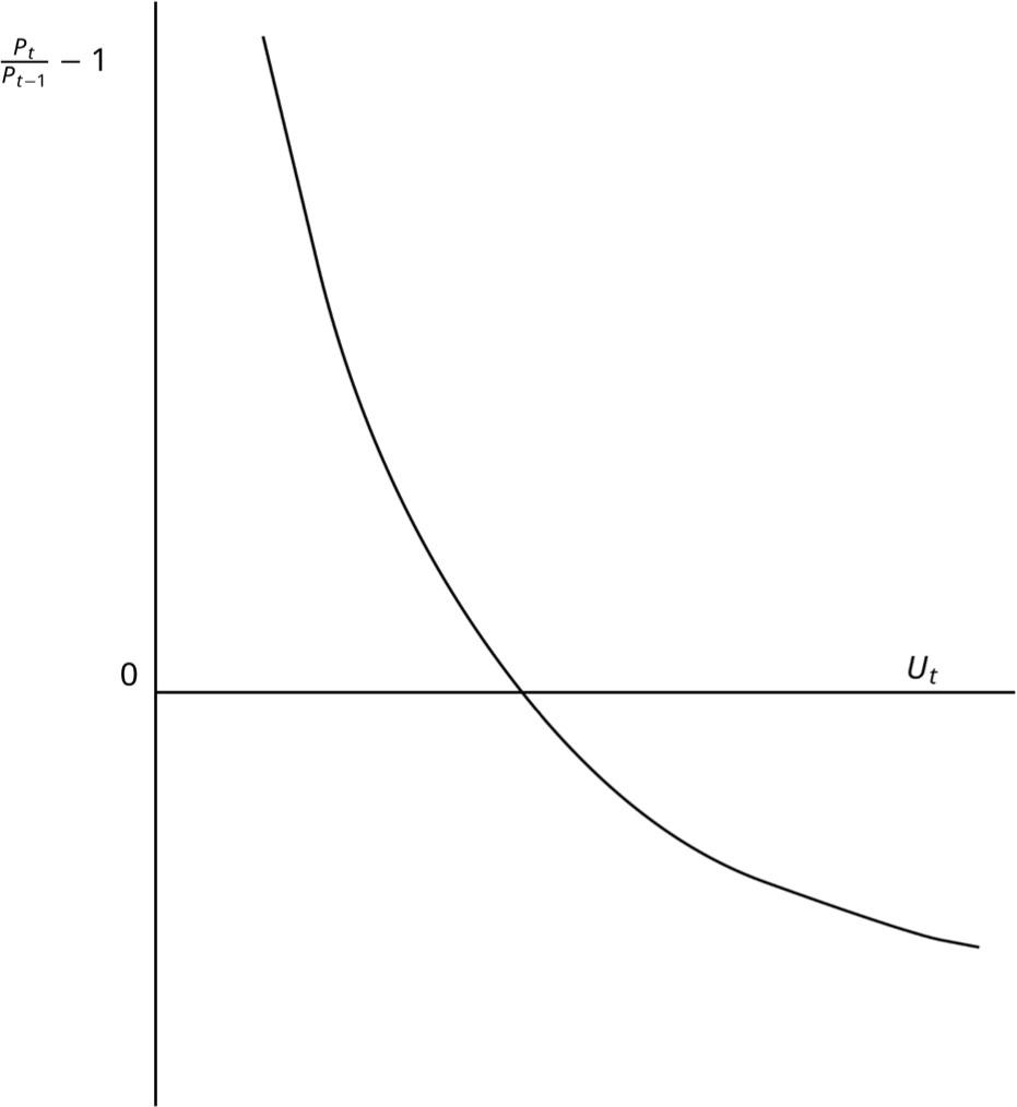
Alternatively, suppose that the nominal wage rate rises. The price of the goods also rises. If the negative real balance effect works, the real aggregate demand increases. Then, the output and the employment increase. Therefore, the higher price or higher inflation rate is accompanied by an increase in employment. Thus, we obtain a negative relationship between the inflation rate and the unemployment rate (positive relationship between the inflation rate and employment) as represented by the Phillips curve. We have shown a negative relationship between the inflation rate and the unemployment rate in the same period given the price in the previous period. Figure 1 depicts an example of the Phillips Curve. Ut denotes the unemployment rate in period t. Figure 1 implies that our model explains the inflation rate between periods t−1 and t by the unemployment rate in period t.
Phillips curve
Let T be the tax revenue other than the taxes for the pay-as-you-go pension system and the unemployment benefits. Then, the budget constraint of the government is G=T, and the aggregate demand is
Given labour productivity y(L) and nominal wage rate W, the price of the goods P1 is determined by Eq. (11). If the government expenditure G increases given T, that is, an increment of the government expenditure is financed by seigniorage, from Eq. (16) employment L increases given the price P1. Then, the Phillips curve in Figure 1 shifts to the left as shown in Figure 2, the employment increases and the unemployment rate decreases given the inflation rate. With increasing returns to scale, y(L) is increasing with respect to L and the prices of the goods fall. However, employment will still increase.
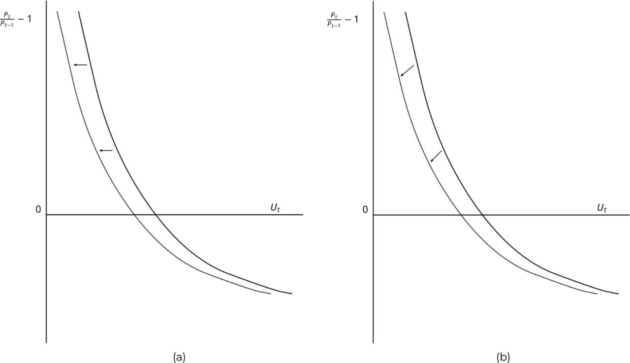
(a) Case of y‘(L)=0 (constant returns to scale) and (b) case of y‘(L)>0 (increasing returns to scale)
The money supply will increase by the difference between government expenditure and the tax. If the increase in the government expenditure is financed by seigniorage, it equals the increase in money supply. Therefore, the fiscal policy in this article is also a monetary policy. It should be called a fiscal-monetary policy. The increase in money supply does not raise the price. Thus, money is not neutral.
Otaki and Tamai (2012) suppose that the low (or high) unemployment rate in a period, for example, period t−1 raises (or lowers) the labour productivity in period t by learning effect. If the unemployment rate in period t−1 increases, the labour productivity in period t falls. Then, from Eq. (11), the price of the goods rises, and the inflation rate from period t to period t+1 falls given the (expected) price of the goods in period t+1. Alternatively, a decrease in the unemployment rate in period t−1 raises the labour productivity in period t. Then, the price of the goods falls, and the inflation rate from period t to period t+1 rises given the (expected) price of the goods in period t+1. Thus, they have shown the negative relation between the unemployment rate in period t−1 and the inflation rate from period t to period t+1,
Their Phillips curve is depicted in Figure 3. Ut–1 denotes the unemployment rate in period t−1.

Phillips curve by Otaki and Tamai (2012)
The thicker curve in Figure 3 means that the low unemployment rate in period t−1 explains the high inflation rate between periods t and t+1 in the model of Otaki and Tamai (2012). The thinner curve shows that the increase in the unemployment rate in period t−1 leads to the higher inflation rate between periods t−1 and t in their model.
We have shown that in a three-period OLG model under monopolistic competition changes in the nominal wage rate bring about the negative relation between the unemployment rate and the inflation rate in the same period. This conclusion is based on the premise of utility maximisation of consumers and profit maximisation of firms. Therefore, we have presented a microeconomic foundation of the Phillips curve. In the future research, we will conduct an empirical analysis of the relationship between the unemployment rate and the rate of inflation and the relationship between the rate of inflation (or the rate of deflation) and consumption expenditures to investigate the effect of the (negative) real balance effect on the shape of the Phillips curve.
There are other ideas that derive the Phillips curve based on the utility-maximising behaviour of consumers and profit-maximising behaviour of firms. Exogenous changes in labour productivity may be one of them. The logic is as follows. If the labour productivity in a period, for example, period t, increases, then the employment decreases and the unemployment rate in period t increases. An increase in labour productivity leads to a decrease in prices given nominal wage rate, and the inflation rate from period t−1 to period t decreases. Alternatively, if the labour productivity in period t decreases, the employment increases, and the unemployment rate in period t decreases. A decrease in labour productivity leads to an increase in prices given nominal wage rate, and the inflation rate from period t−1 to period t increases.
About the traditional discussion of real balance effects, refer Pigou (1943) and Kalecki (1944).