

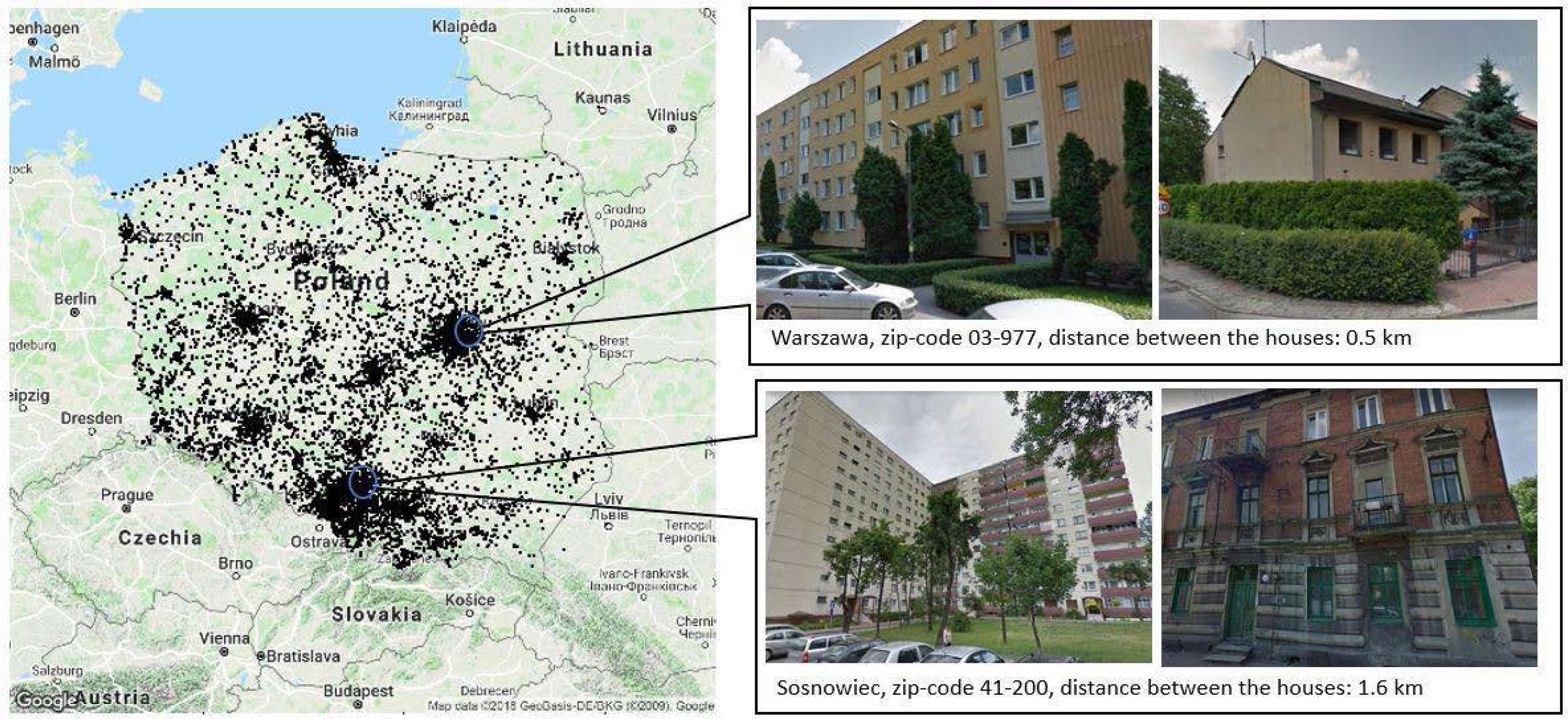
Fig. 1
Examples of extremely different houses located in the same zip code and residents of which have the same expected claim frequency by the current insurer’s model.
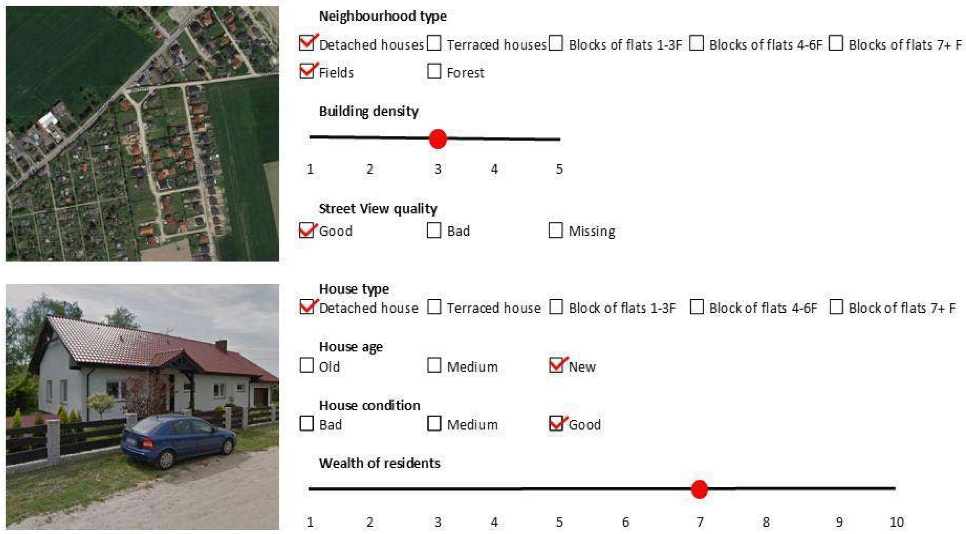
Fig. 2
Features annotated from Google Satellite View and Google Street View image of a particular address.
Tab. 1
Statistics for seven newly created variables—original granularity, inter-rater reliability of 4 selected annotators on the common set of 500 observations and significance in our risk model after applying necessary simplifications.
| Variable | Original granularity | Inter-rater reliability | Risk model | ||
|---|---|---|---|---|---|
| Fleiss’ kappa | Interpretation | Granularity after simplification | p-value | ||
| Neighbourhood type | Seven types, multi-choice | 0.52 | Moderate agreement | 2 | 00.01 |
| Building density | Scale 1–5 | 0.50 | Moderate agreement | Not significant | |
| Street View quality | Good/bad/missing | 0.79 | Substantial agreement | 2 | 00.02 |
| House type | Five types, single-choice | 0.69 | Substantial agreement | 2 | 00.01 |
| House age | Scale 1–3 | 0.51 | Moderate agreement | 2 | 00.03 |
| House condition | Scale 1–3 | 0.54 | Moderate agreement | 2 | 00.04 |
| Wealth of residents | Scale 1–10 | 0.32 | Fair agreement | Not significant | |
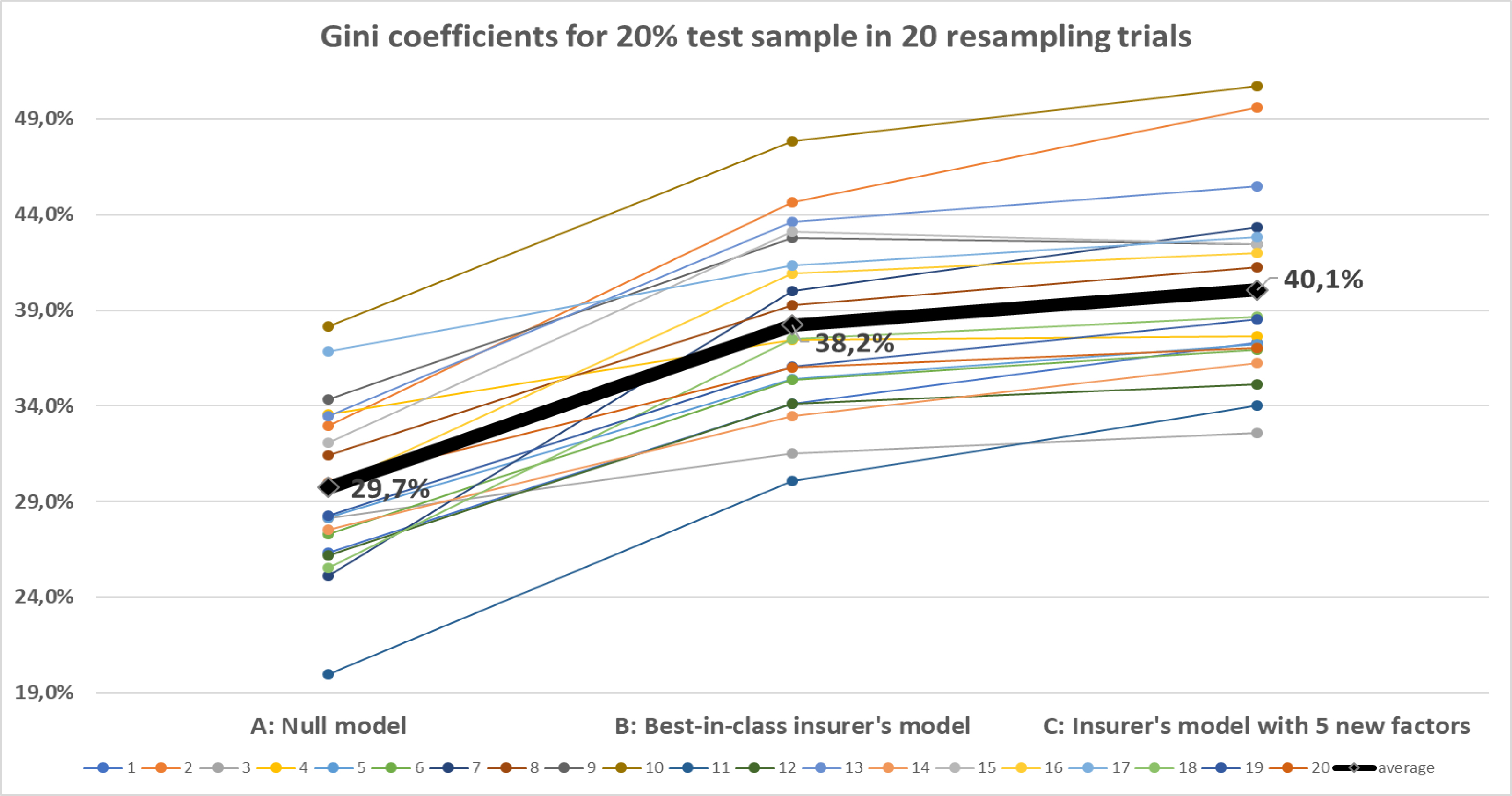
Fig. 3
Gini coefficients obtained on 20% test sample in 20 bootstrapping trials from the null model (A), the best-in-class insurer’s model (B) and our model with newly created variables (C).
Tab. 2
Summary statistics of the dataset—before and after cleansing.
| Original database | After data cleansing | |
|---|---|---|
| Number of polices | 20,000 | 19,871 |
| Risk exposure | 11,349 | 11,209 |
| MTPL PD claim count | 571 | 570 |
| Observed MTPL PD frequency | 5,03% | 5,09% |
Tab. 3
Data for calculation of X2 statistic for hypothesis verification whether claims in our dataset follow the Poisson distribution. On average λ = 3.9% and the corresponding X2 = 0.08 with 1 degree of freedom.
| Number of claims | Observed exposure (O) | Expected prob.P(X = k) | Expected exposure (E) | (E – O)2/E |
|---|---|---|---|---|
| 0 | 10,784 | 96% | 10,785 | 0,00 |
| 1 | 417 | 4% | 416 | 0,01 |
| 2 | 7 | 0% | 8 | 0,08 |
| All | 11,209 | |||
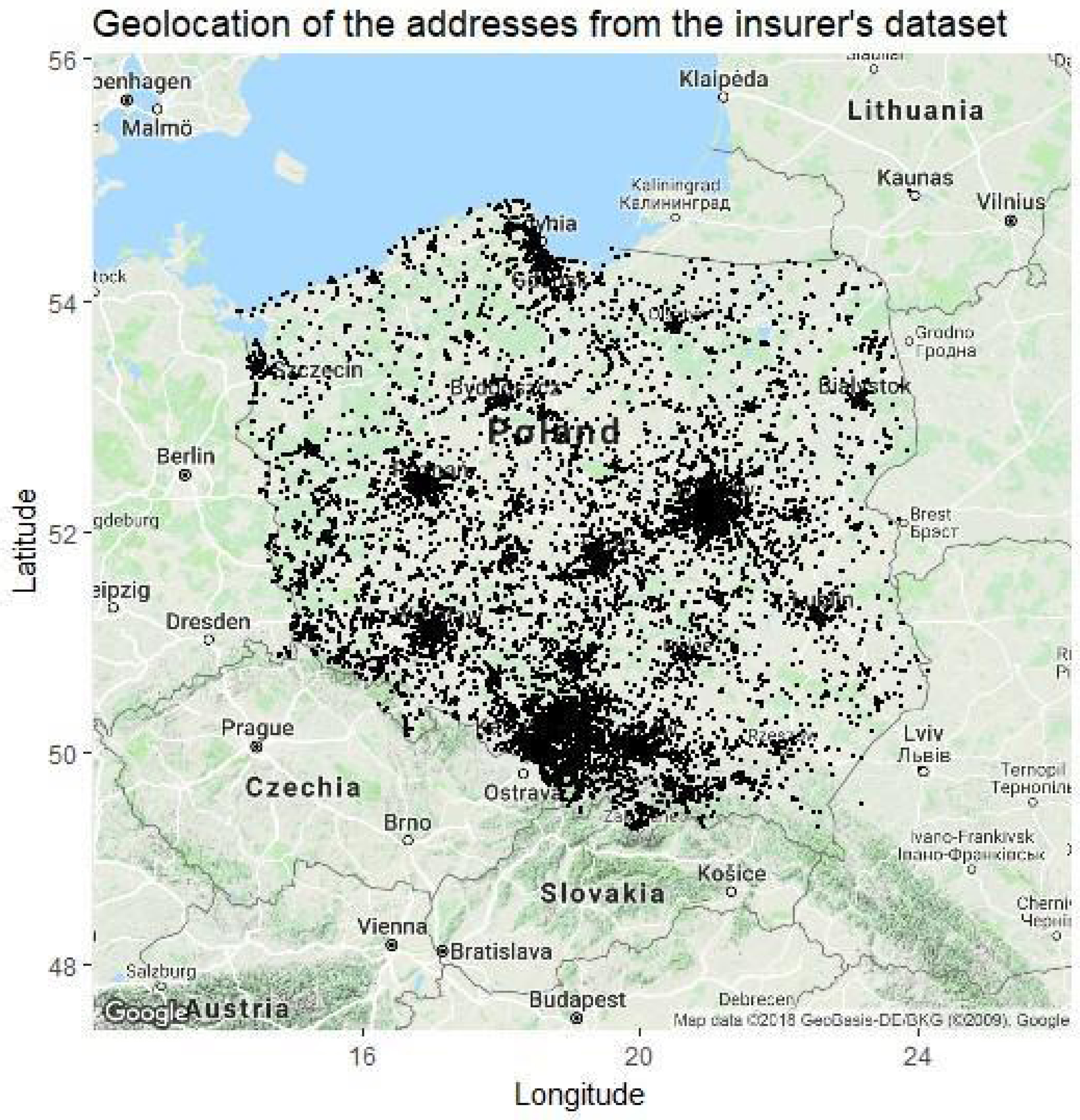
Fig. 4
Geolocation of the addresses from the dataset examined in this paper.
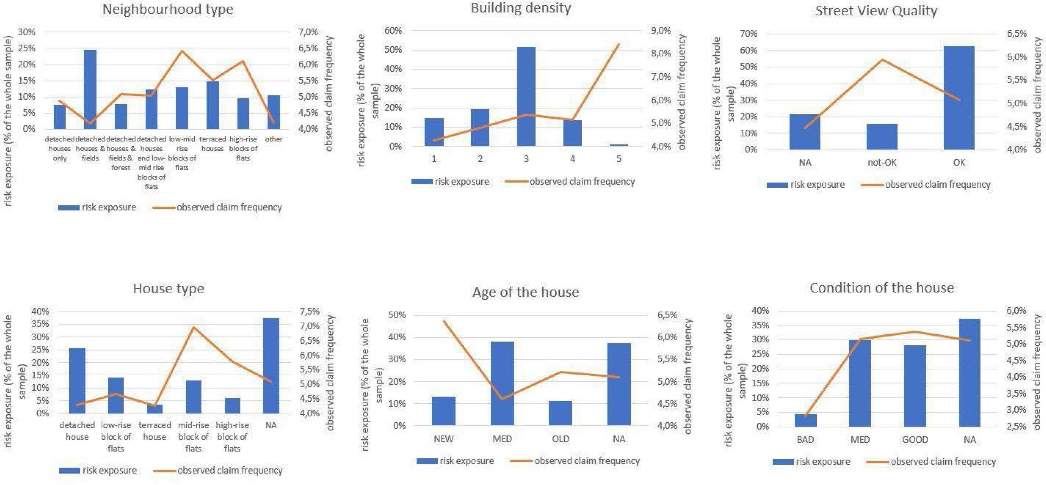
Fig. 5
Distribution of labels and corresponding observed claim frequency for the variables generated for this study.
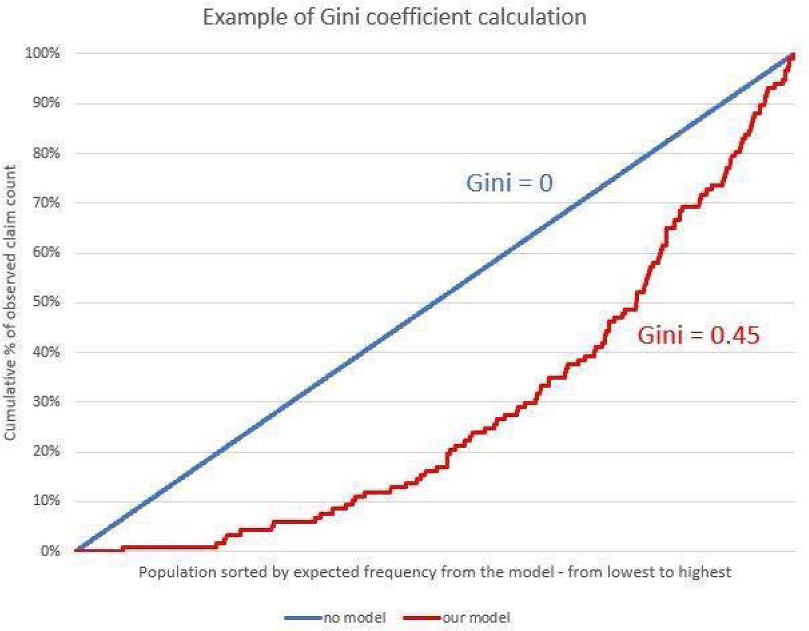
Fig. 6
Illustration of the Gini coefficient computation for one of the bootstrapping trials.