

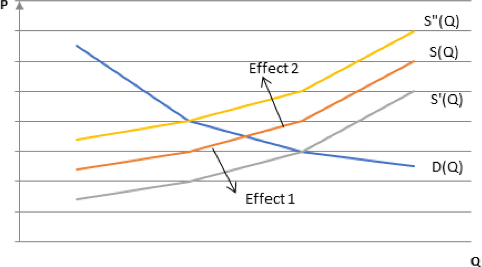
Graph 1
Two BIG’s effects on labour market. Source: own elaboration.
Tab. 1
Monthly basic income guarantee per capita equal to current aggregated social services and tax allowances
| Adult | Child (<18) | Poverty line for an individual | |
|---|---|---|---|
| Finland | €527 | €316 | €1074 |
| France | €456 | €100 | €909 |
| Italy | €158 | €158 | €737 |
| Great Britain | £230 | £189 | £702 |
[i] Source: Elaboration based on: OECD (2017). Basic Income As a Policy Option: Can it add up?. Policy Brief on The Future of Work, OECD Publishing. On line. Access 06.02.2018. https://www.oecd.org/els/emp/Basic-Income-Policy-Option-2017.pdf.
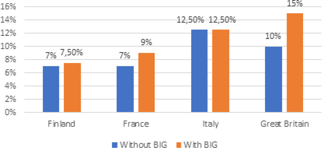
Graph 2
Poverty level currently and after implementing the basic income guarantee. Source: own elaboration* based on: OECD (2017). Basic Income As a Policy Option: Can it add up?. Policy Brief on The Future of Work, OECD Publishing. On line. Access 06.02.2018. https://www.oecd.org/els/emp/Basic-Income-Policy-Option-2017.pdf
*The graph is only an approximation of a table present in (OECD 2017). Its exact model would require repeating the whole simulation, as the authors present in the report only approximated bars.
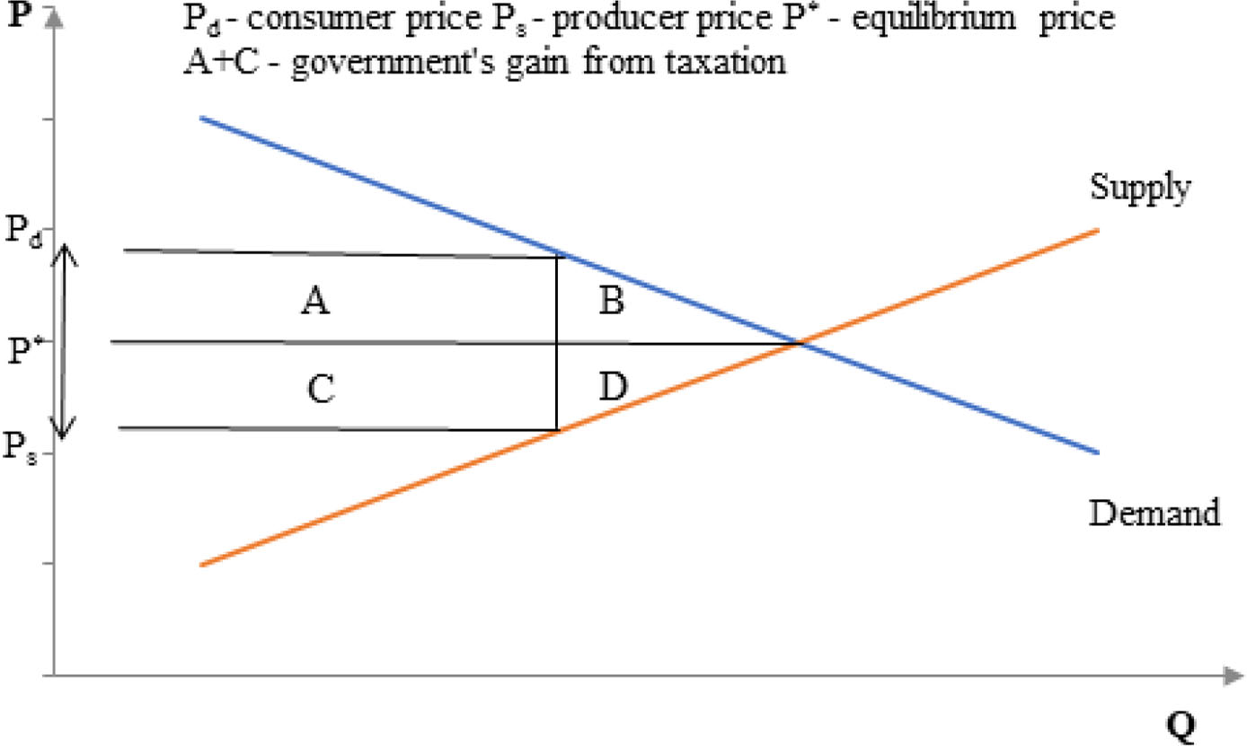
Graph 3
Deadweight loss caused by taxation. Source: own elaboration based on: Varian (2010). Intermediate Microeconomics. A Modern Approach. Eighth Edition. W. W. Norton & Company, New York, London, 305.
Tab. 2
Work and welfare – a possible situation 1
| Gross Income | Tax | Transfers | BIG | Net Income | |
|---|---|---|---|---|---|
| Person 1 | $500 000 | $136 800 | $0 | $0 | $363 200 |
| Person 2 | $200 000 | $46 800 | $0 | $0 | $153 200 |
| Person 3 | $100 000 | $16 800 | $0 | $0 | $83 200 |
| Person 4 | $10 000 | $0 | $6 000 | $0 | $16 000 |
| Person 5 | $0 | $0 | $16 000 | $0 | $16 000 |
| Together: $200 400 | Together: $22 000 | Together: $0 | |||
| Government’s net revenue: $178 400 | |||||
[i] Source: Elaboration based on: Munger (2015b). One and One-Half Cheers for a Basic-Income Guarantee: We Could Do Worse, and Already Have. The Independent Review, Vol. 19, No. 4.
Tab. 3
Work and welfare – possible situation 2
| Gross Income | Tax | Transfers | BIG | Net Income | |
|---|---|---|---|---|---|
| Person 1 | $500 000 | $153 120 | $0 | $16 000 | $362 800 |
| Person 2 | $200 000 | $57 120 | $0 | $16 000 | $158 880 |
| Person 3 | $100 000 | $25 120 | $0 | $16 000 | $90 880 |
| Person 4 | $10 000 | $5 200 | $0 | $16 000 | $20 800 |
| Person 5 | $0 | $3 200 | $0 | $16 000 | $12 800 |
| Together: $243 760 | Together: $0 | Together: $80 000 | |||
| Government’s net revenue: $163 760 | |||||
[i] Source: Elaboration based on: Munger (2015b). One and One-Half Cheers for a Basic-Income Guarantee: We Could Do Worse, and Already Have. The Independent Review, Vol. 19, No. 4.
Tab. 4
Influence of the basic income guarantee
| Predicted positive effects | Predicted negative effects |
|---|---|
| It might increase work incentives (Effect 1#) | Might increase work disincentives (Effect 2) |
| As a cash transfer much more efficient than in-kind | In case of keeping budget-neutrality a very small size of a payment |
| Will increase stability on labour market | A bigger payment requires tax increase → a work disincentive |
| Lower administrative costs than in current programmes | Higher taxes → a bigger deadweight loss |
| Less exclusive and humiliating for recipients | After BIG implementation the needy might loose |
Source: Elaboration based on literature quoted in the section.
# “Effect 1” and “Effect 2” refer to possible BIG effects on labour market, presented on Graph 1.
Tab. 5
Labour supply changes due to the negative income tax
| Worked hours (yearly) | Employment rate | |
|---|---|---|
| Husbands | −89 (−5%) | −0.3 (−3.5%) |
| Wives | −117 (−21.1%) | −0.6 (−22.5%) |
| Single female heads | −123 (−13.2%) | −0.7 (−15.7%) |
| Youths | −173 (−22.2%) | −0.9 (−20%) |
| In parentheses percentage change | ||
[i] Source: Elaboration based on: Robins (1985). A Comparison of the Labor Supply Findings from the Four Negative Income Tax Experiments. The Journal of Human Resources, Vol. 20, No. 4, 567–582.
Tab. 6
Average substitution and income effects from all four experiments
| Substitution effect (for $/h) | Income effect (for $1 000) | |
|---|---|---|
| Husbands | 45 (0.08) | −25 (−0.10) |
| Wives | 101 (0.17) | −22 (−0.06) |
| Single female heads | 78 (0.13) | −55 (−0.16) |
| Substitution and income elasticities in parentheses | ||
[i] Source: Elaboration based on: Robins (1985). A Comparison of the Labor Supply Findings from the Four Negative Income Tax Experiments. The Journal of Human Resources, Vol. 20, No. 4, 567–582.
Tab. 7
Poverty rate and poverty gap in Iran (percentage)
| Year | Poverty rate | Poverty gap | ||||||
|---|---|---|---|---|---|---|---|---|
| Countryside | Cities | Teheran | Total | Countryside | Cities | Teheran | Total | |
| 2009 | 13.4 | 9.8 | 6.2 | 10.2 | 4.0 | 2.6 | 1.3 | 2.8 |
| 2010 | 10.3 | 7.2 | 5.6 | 7.8 | 2.9 | 1.8 | 1.1 | 2.0 |
| 2011 | 6.3 | 5.2 | 2.8 | 5.2 | 1.5 | 1.1 | 0.7 | 1.2 |
| 2012 | 5.0 | 5.4 | 4.4 | 5.1 | 1.0 | 1.1 | 0.8 | 1.0 |
[i] Source: Elaboration based on: Salehi-Isfahani (2014). Iran’s Subsidy Reform from Promise to Disappointment. Policy Perspective, No. 13. Economic Research Forum, 7.
Tab. 8
Inequalities in Iran (Gini index)
| Year | Expenses per capita | Income per capita |
|---|---|---|
| 2009 | 0.421 | 0.414 |
| 2010 | 0.415 | 0.414 |
| 2011 | 0.382 | 0.367 |
| 2012 | 0.375 | 0.367 |
[i] Source: Elaboration based on: Salehi-Isfahani (2014). Iran’s Subsidy Reform from Promise to Disappointment. Policy Perspective, No. 13. Economic Research Forum, 7.