

1. Introduction
The use of base isolation (BI) systems to reduce seismic force demands on buildings has been implemented for decades, in both newly constructed and existing buildings. The concept behind base isolation is primarily to lengthen the natural period of structures and enhance energy dissipation. Several studies have reported that this can be achieved by placing laterally flexible elements between the foundation and the upper structure (Kelly & Konstantinidis, 2011; Martelli & Forni, 2010). High-damping rubber bearings (HDRB), lead-rubber bearings (LRB), and friction isolation systems (FIS) are well-known BI technologies that have been used in numerous constructions worldwide. For the upper structure, the BI system can reduce inter-story drift, thereby improve seismic performance and minimize potential damage to structural elements. The acceleration response of the upper structure can also be reduced, offering more protection to non-structural components such as furniture and vibration-sensitive devices, while providing greater comfort to occupants during small to medium earthquakes. In general, the BI system is designed to ensure that the upper structure remains intact after the maximum considered earthquake, thereby eliminating the potentially high costs of rehabilitation and ensuring the continuity of building functions, especially in critical facilities such as hospitals, power plants, and other vital infrastructure.
Several studies have demonstrated the effectiveness of BI systems for seismic protection of buildings in the literature, investigating the performance of either conventional-commercial BI devices or newly developed low-cost devices (Imran et al., 2021; Tena-Colunga & Parra-García, 2024; Shiravand et al., 2022; Kanbir et al., 2020; Galano et al., 2021; Sheikh et al,. 2025; Pianese et al., 2024; Habieb et al. 2022; Ibrahim & Mohamad, 2024; Ahmed et al., 2024). Despite the widespread implementation of the BI system, it was considered effective only when used in low- to medium-rise buildings standing on medium to hard soil. There is still doubt about the use of the BI system in high-rise buildings and buildings constructed on soft soils due to the risk of resonance phenomenon because the period of the soft soil can be as large as the period of the isolated structure. Zhuang et al. (2019) performed a shaking table test to evaluate the performance of the BI system in a building model founded on multi-layered soft soil. The study reported that the soft soil profile might increase the dominant period of the site and therefore be close to the effective isolation system’s period, which generated structural resonance. Hassan & Pal (2018) have investigated the effectivity of the BI system in different soil conditions. It was revealed that the inter-story drift increased with the increased flexibility of the soil, which demonstrated the deficiency of the BI system in soft soil conditions.
On the other hand, several studies demonstrated the benefit of using the BI system in buildings standing on soft soil. Almansa et al. (2020) have reported a case study on an isolated building standing on soft soil in Shanghai. It was concluded that the BI system, when properly designed, can be an effective seismic protection for mid-height RC buildings on soft soil and located in medium seismicity regions. Pérez-Rocha et al (2021) performed comprehensive NLTH analysis on the application of the BI system on mid-rise buildings on soft soil in Mexico City. The study revealed that the BI system applied in mid-rise buildings on soft soil performed satisfactorily if the dominant site period is larger than the fundamental structural period and simultaneously much shorter than the effective isolation period. These conclusions may support the promotion of the BI system in regions with soft soil, which are often located in many densely populated urban areas. Furthermore, as the soil-structure interaction (SSI) effect is pronounced in the case of soft soil, the design and analyses of the BI system for buildings founded on soft soil may involve advanced modelling and simulation to ensure the optimal performance of the BI system.
In real practice, the SSI effect is often neglected, particularly in the structural seismic analyses of low to mid-rise buildings. Common seismic analysis is generally performed based on the simplified assumption that the structure stands on a rigid rock, thus the seismic wave is transferred from the bedrock to the base of the structure without being affected by soil flexibility. This approach may lead to a conservative design of the upper structure. On the other hand, in the case of long-period structures such as high-rise buildings and base-isolated buildings, the SSI effect may generate detrimental effects. Thus, the SSI modelling is important to be considered in such cases.
Several modelling strategies to consider the SSI effect have been introduced in many studies. The first model is the indirect approach where a series of translational or rotational spring-dashpot models are used to represent the horizontal and vertical stiffness and damping properties of the soil profile that are in contact with the piles or the base of the upper-structure (Madani et al., 2015; Mahmoud et al., 2018; Farajian et al., 2017; Behnamfar & Banizadeh, 2016; Soneji & Jangid, 2008; Bakhtiari & Bargi, 2020). The second model is the direct approach in which the upper structure and the soil profile are modelled and analysed simultaneously in the finite element model (Fathi et al., 2020; Altiok & Demir, 2021; Genç et al., 2023; Hasan & Younos, 2023; Shabani & Kioumarsi, 2023; Casolo et al., 2017; Luo et al., 2016; Van Nguyen et al., 2017). The latter requires expensive computational effort and may not be suitable for large nonlinear scale time-history analysis.
Several studies investigating SSI effects in soft soil have reported that the longer the fundamental period of the structure, the more earthquake base shear was generated. It was also followed by an increase in the acceleration response and the inter-story drift (Almansa et al., 2020; Karabork et al., 2014). In another study, Yanik et al (2023) performed large-scale NLTH analysis using 15 ground motion records in various locations. In line with general assumptions, the SSI effects were found significant in soft soil case and barely present in the case of dense soil. Even though the floor displacement could be reduced by the application of BI, the effectiveness of the BI system was found to decrease when SSI was considered.
Those findings reveal the importance of advanced numerical modelling in the analysis of base-isolated buildings founded on soft soil, taking into account the SSI effect. As the study on the effectiveness of the BI system in soft soil sites is still limited, more case studies are still required to demonstrate the benefit of using the BI system in the case of soft soil using advanced analysis and proper design. In this study, a 13-story reinforced concrete (RC) building model founded on soft soil was considered. Seismic performance evaluation was performed in accordance with ASCE 41-17 through a series of nonlinear time history analyses, considering the effect of SSI and the implementation of LRB-based BI system.
The remainder of this paper is organized as follows. Section 2 describes the methodology, including the building model, material properties, design and modelling of the lead–rubber bearing (LRB) isolation system, plastic hinge modelling, and the soil–structure interaction (SSI) approach. Section 3 presents the modal analysis results of the considered structural models. Section 4 describes the selection and scaling of ground motions used in the nonlinear time-history analysis. Section 5 presents and discusses the results of the nonlinear time-history analysis, including base shear, performance of the BI system, inter-story drift, and acceleration response. Finally, Section 6 summarizes the main findings and conclusions of the study.
2. Methodology
2.1. Description of The Building Model and Site Under Study
The building under study, as shown in Figure 1 is an existing 13-story RC building with a moment-resisting frame (MRF) system founded on soft soil located in Surabaya, East Java, Indonesia. The building has a regular 27.6 × 30 m2 plan and a uniform section along its height, as shown in Figure 2 and Figure 3. The height of each story is 3.75 m; thus, the total height of the building becomes 48.75 m. The building was designed based on the previous national seismic-design code dating back to 2012, which is equivalent to ASCE 7-10.
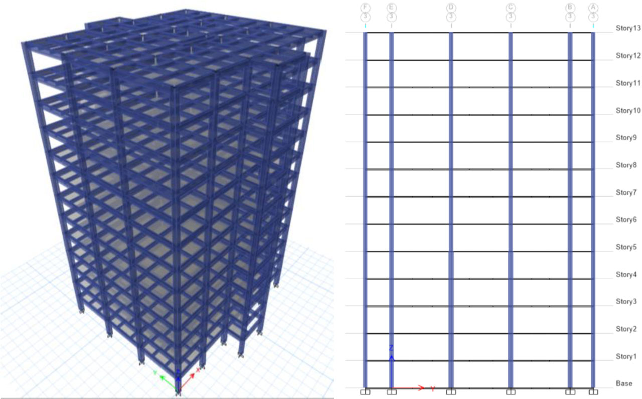
Figure 1:
(a) Isometric view and (b) Cross section of the building model
For the primary structural elements, concrete with a compressive strength of 33.20 MPa was used, while the reinforcing bars had a yield stress of 400 MPa. The dimensions and reinforcement details of beam and column elements are presented in Figure 4 and Figure 5. The building stands on a spun-pile foundation system with an average depth of 25 m.
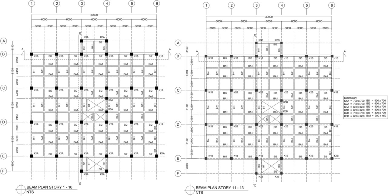
Figure 2:
Plan view of the building and the indication of the primary beams for (a) 1st-10th floor and (b) 11th-13th floor
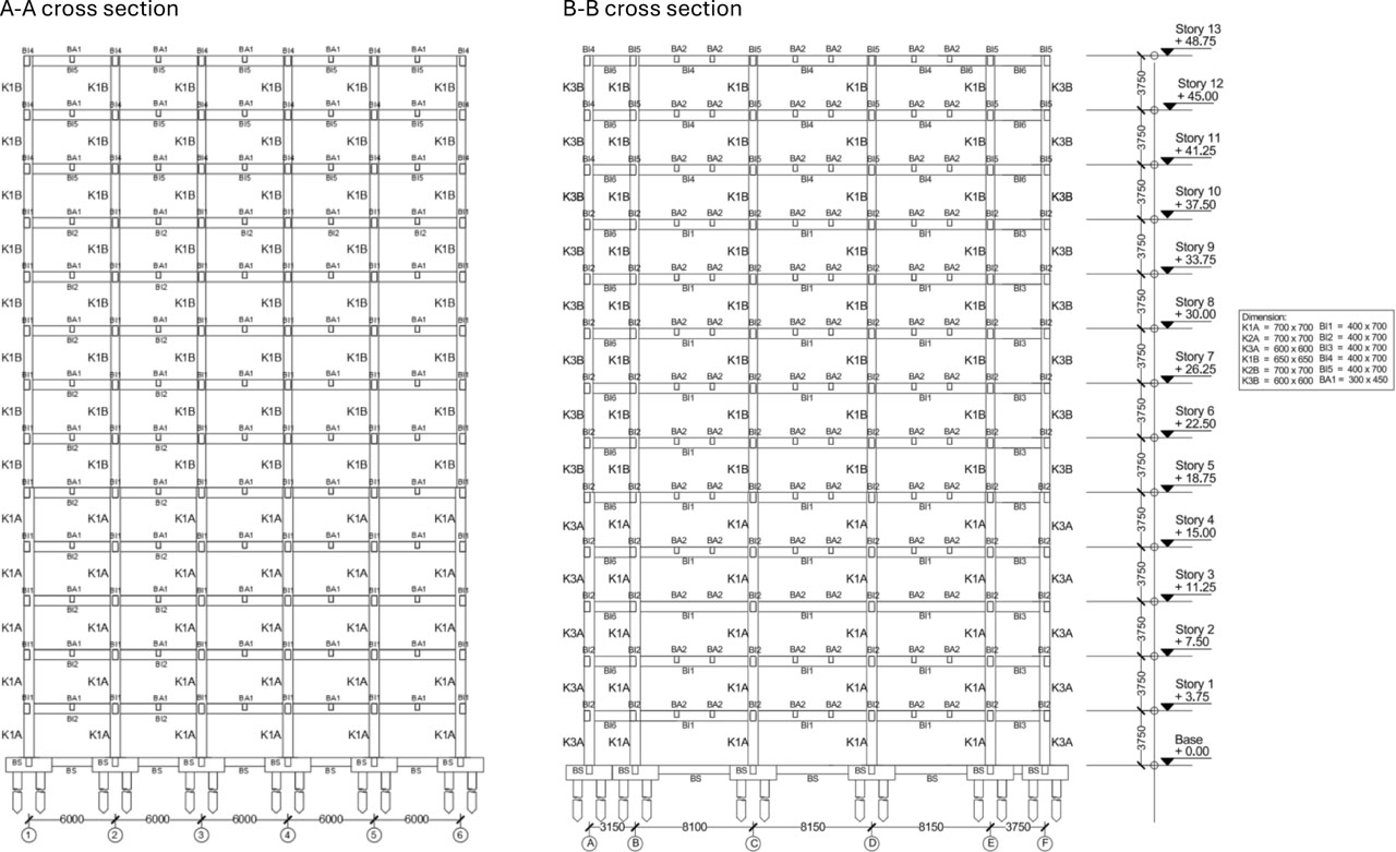
Figure 3:
Cross sections of the building and indication of column dimensions
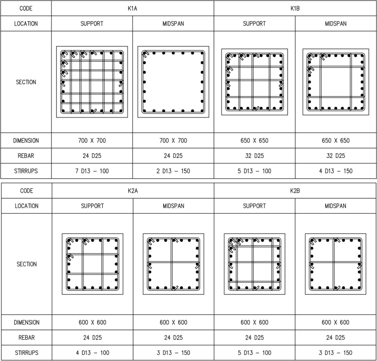
Figure 4:
Reinforcement detail of the RC columns
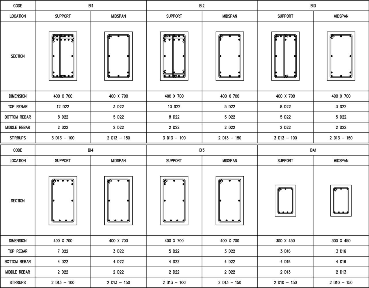
Figure 5:
Reinforcement detail of the primary RC beams
Table 1:
Site soil profile
| Depth | di (m) | Ni (N-SPT) | di / Ni |
|---|---|---|---|
| 1 | 1 | 4 | 0.25 |
| 2 | 1 | 1.67 | 0.6 |
| 3 | 1 | 0.83 | 1.2 |
| 4 | 1 | 0.56 | 1.8 |
| 5 | 1 | 0.56 | 1.8 |
| 6 | 1 | 3.5 | 0.29 |
| 7 | 1 | 7 | 0.14 |
| 8 | 1 | 8 | 0.13 |
| 9 | 1 | 9 | 0.11 |
| 10 | 1 | 10 | 0.1 |
| 11 | 1 | 10 | 0.1 |
| 12 | 1 | 11 | 0.09 |
| 13 | 1 | 11 | 0.09 |
| 14 | 1 | 12 | 0.08 |
| 15 | 1 | 13 | 0.08 |
| 16 | 1 | 13 | 0.08 |
| 17 | 1 | 14 | 0.07 |
| 18 | 1 | 18 | 0.06 |
| 19 | 1 | 22 | 0.05 |
| 20 | 1 | 22 | 0.05 |
| 21 | 1 | 22 | 0.05 |
| 22 | 1 | 19 | 0.05 |
| 23 | 1 | 18 | 0.06 |
| 24 | 1 | 18 | 0.06 |
| 25 | 1 | 19 | 0.05 |
| Total | 25 | 7.42 |
Based on the average N-SPT up to a depth of 25 m, the soil profile is classified as Site Class E (soft soil) in accordance with ASCE 7-16 Table 20.3-1. The average SPT value (Navg) is calculated from the soil profile data presented in Table 1, resulting in a value of Navg = 7.42, which is less than 15. This value satisfies the criterion for Site Class E, which corresponds to soft soil conditions. Spectral responses of the site with the return periods of 250, 1000, and 2500 years were analysed as the basis of the seismic isolation design and the selection of suitable ground motions in NLTH analysis of the existing building, as shown in Figure 6.
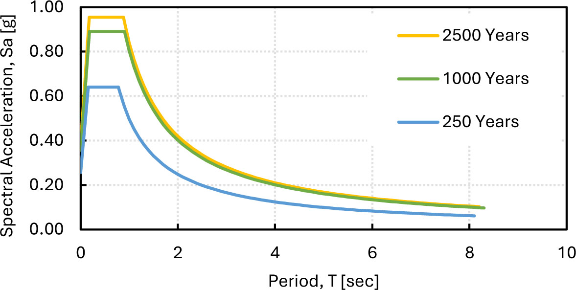
Figure 6:
Spectral response of the site under study for earthquakes with 250, 1000, and 2500 years of return period
To evaluate the effectiveness of BI implementation and SSI effect, four models were considered in this study, as follows:
FB : fixed-base model without soil structure interaction,
BI : base-isolated model without soil structure interaction,
FB-SSI : fixed-base model with soil structure interaction,
BI-SSI : base-isolated model with soil structure interaction.
2.2. Design and Modelling of Lead Rubber Bearing (LRB) Isolation System
The BI system was designed using LRB isolators based on the assumption of a single degree of freedom (SDOF) in which the upper structure is considered a single rigid mass system. The BI system was designed to withstand a maximum considered earthquake (MCEr) with 2500 years of return period. The target isolation period was set to twice that of the fundamental period of the initial fixed-base structure. Two sizes of LRB were considered to accommodate proportional service loads at the exterior and interior columns, as indicated in Figure 7 and Table 2
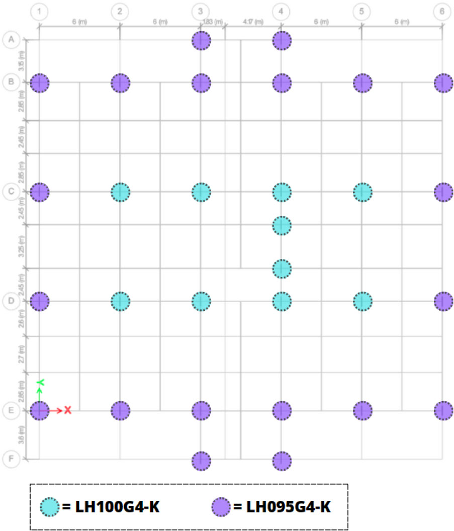
Figure 7:
Configuration of the LRB isolators at the base of the building
Table 2:
LRB isolator properties
| No | Isolator parameters | LRB Interior | LRB Exterior |
|---|---|---|---|
| 1 | Isolator type | LH100G4-K | LH095G4-K |
| 2 | Maximum vertical load, Pmax (kN) | 9454.81 | 8110.73 |
| 3 | Bearing diameter, DB (mm) | 1000 | 950 |
| 4 | Lead plug diameter, DL (mm) | 250 | 240 |
| 5 | Total thickness of rubber, Tr (mm) | 201 | 198 |
| 6 | Rubber shear modulus, Gr (MPa) | 0.385 | 0.385 |
| 9 | σload (MPa) | 12.84 | 12.22 |
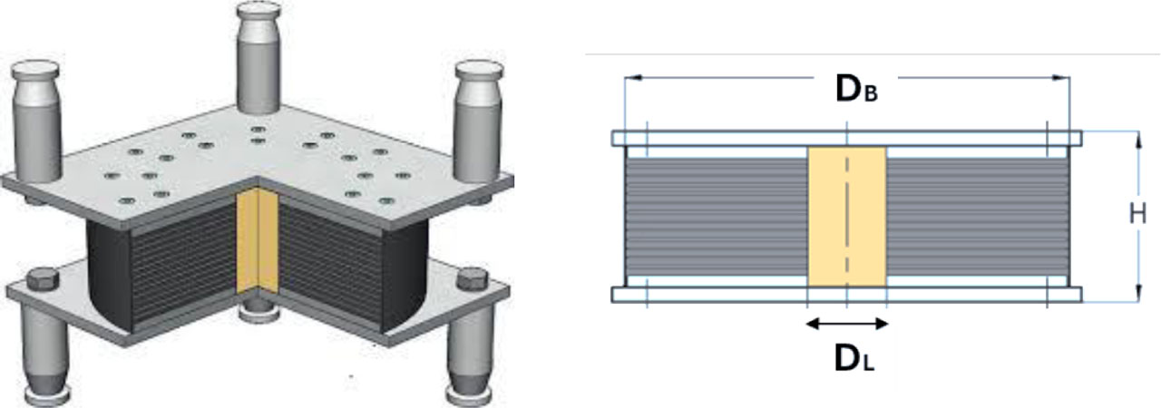
Figure 8:
(a) 3D isometric view, and (b) lateral-section of LRB isolator (Source: ISOSISM®)
The dimensions and mechanical properties of the LRBs are presented in Table 2 and Figure 8. Several performance parameters were controlled during the design to ensure the stability of the BI devices, including peak horizontal displacement and critical compressive and tensile force. Even though the tensile strength of the BI devices can be evaluated, the BI system is generally not expected to undergo tensile force. Therefore, an overturning of the superstructure should be avoided during an earthquake event.
For numerical analysis, the bilinear model of the LRB isolators was defined using bilinear parameters as presented in Table 3, where the definition of each parameter was described by Figure 9. As the dissipative device, such parameters resulted in a damping ratio at the designed displacement of approximately 30%. In real practice, the bilinear mode should be calibrated with the experimental data of the cyclic shear test on the isolator.
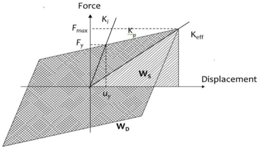
Figure 9:
Schematic bilinear model of the LRB isolators
2.3. Plastic Hinge Model of the RC Columns and Beams
In the nonlinear time-history (NLTH) analysis, the building performance strongly depends on the modelling strategy of the plastic hinges on the seismic-resisting structural elements. The properties of the plastic hinges on the RC beams and columns were defined based on ASCE 41-17, where the curvature-moment relationship is defined through the parameters a, b, c, and ultimate limit, as shown in Figure 10. Those parameters of the plastic hinges were computed based on the installed steel reinforcement on the RC beam and columns, as per ASCE 41-17.
Point A is the unloaded condition. Path A to B represents the linear elastic behaviour, with point B where the first yielding occurred and still no permanent element deformation occurred until this point. Path B to C represents the strain-hardening phase until the ultimate strength capacity of the element is reached at point C. Path C to D represents the initial failure and instability of the element. Path D to E represents the residual strength of the element, with point E being considered a complete failure of the element. The acceptance criteria for plastic hinge rotations are categorized into three levels: (i) immediate occupancy, (ii) life safety, and (iii) collapse prevention, all situated between Points B and C. During the NLTH analysis, if a hinge is found at Immediate Occupancy (IO), indicating minor damage, maintaining most of the element’s original stiffness and strength. If the hinge is at Life Safety (LS), the element has incurred damage, altering its stiffness without severe damage to the element. At Collapse Prevention (CP), the element experiences significant damage, leading to a complete change in stiffness.
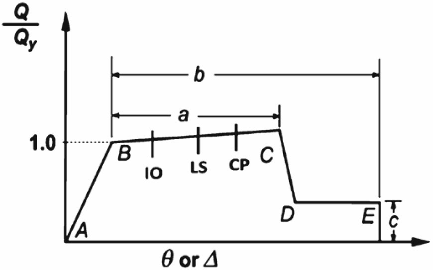
Figure 10:
Schematic curvature-moment relationship model as per ASCE 41-17
The relative distance of the plastic hinge in beams was assumed 0.05L and 0.95L, while in columns was assumed 0.1L and 0.9L, where L is the length of the element. The bending moment plastic hinges were specified in beams, whereas columns are specified with moment-plastic hinges that consider axial forces. In SAP 2000, the user should set firstly the considered shear force value (V) for the beams and axial force value (P) for the columns: the V value for the beam elements corresponds to the force due to the considered seismic action while the P value for the column elements corresponds to the gravitational load in seismic combination (1.0 dead load + 0.25 live load).
2.4. Model of Soil-structure Interaction (SSI)
The present study used an indirect approach to model the SSI where a series of translational spring models are used to represent the horizontal and vertical stiffness of the soil profile that is in contact with the structures. In the case of a building standing on a depth foundation such as a pile system, the spring models were attached to the piles with constant spacing, as shown in Figure 11. This approach is widely used due to its computational efficiency and numerical stability, particularly in nonlinear time-history analysis (NLTHA) of large-scale structures.
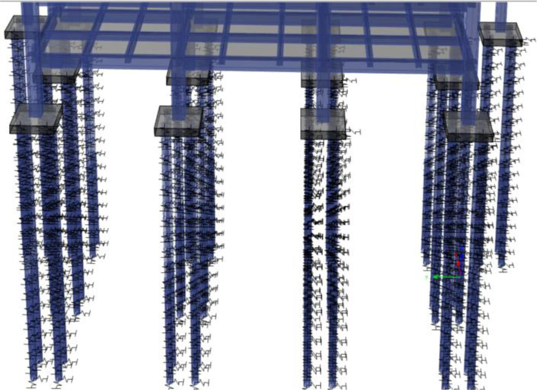
Figure 11:
Representative spring models to consider the SSI effect in SAP 2000
The foundation soil was assumed to remain elastic during the earthquake excitation. This assumption was adopted to simplify the soil–structure interaction (SSI) modelling by considering constant stiffness properties and neglecting soil damping effects. Such a simplification allows for improved computational efficiency and numerical stability, particularly in nonlinear time-history analyses involving complex structural behaviour. Moreover, this approach is consistent with commonly adopted practices in simplified SSI modelling, where the soil is represented using linear elastic springs to capture the global interaction effects (Behnamfar & Banizadeh, 2016; Madani et al., 2015; Mahmoud et al., 2013). In such approaches, the primary objective is to capture the overall dynamic response of the system rather than detailed nonlinear soil behaviour.
It should be noted that energy dissipation in the system is implicitly accounted for through a global damping ratio of 5%, which is consistent with the equivalent viscous damping commonly adopted in seismic response spectrum analysis and design codes. This damping ratio represents the combined effects of material damping, structural hysteresis, and other sources of energy dissipation in the system. Therefore, although soil damping is not explicitly modelled, the overall damping behaviour of the system is reasonably represented for the purpose of evaluating the global seismic response. Consequently, the adopted modelling approach is considered adequate for evaluating the comparative influence of SSI and base isolation on the overall seismic response of the structure. Furthermore, the linear spring constants were evaluated using established formulations proposed by Sosrodarsono and Nakazawa (1983) as presented in Equations (1)–(4).
Where:kh - stiffness of the horizontal spring attached to the pile (stiffness/spacing),
kv – stiffness of the vertical spring attached to the pile,
D – diameter of pile,
E0 – elastic modulus of soil,
N – SPT blow count,
y – lateral soil deformation ≈ 1 cm,
Ep – Elastic modulus of pile,
Ap – cross-section area of pile,
α – pile coefficient of precast concrete,
l – depth of pile.
The calculated soil spring parameters used in the SSI model are summarized in Table 4. The table presents the variation of soil properties with depth, including N-SPT values, deformation modulus (E0), pile coefficient (α), and the corresponding horizontal (kh) and vertical (kv) spring stiffness values. The results show that both Kh and Kv generally increase with depth, reflecting the increase in soil stiffness associated with higher N-SPT values. The relatively low stiffness values in the upper layers are consistent with soft soil conditions (Site Class E), while deeper layers exhibit higher stiffness due to denser soil conditions.
The pile foundation system is explicitly defined in the SSI model, consisting of a total of 128 piles with a diameter of 0.6 m and a centre-to-centre spacing of 1.6 m. These parameters are incorporated into the calculation of spring stiffness and the distribution of soil springs along the pile depth. The spacing between piles influences the interaction area of each pile with the surrounding soil, thereby affecting the equivalent stiffness representation in the SSI model.
Finally, the depth-dependent spring stiffness values are implemented as discrete translational springs along the pile elements in the numerical model. This modelling strategy enables the SSI system to capture the variation of soil stiffness along depth while maintaining computational efficiency. Therefore, the adopted approach provides a realistic yet practical representation of the interaction between the soil, foundation, and superstructure for seismic response evaluation.
Table 4:
Summary of soil spring parameters for SSI modelling
| Depth [m] | N-SPT | Deformation modulus | α | Horizontal spring stiffness | Vertical spring stiffness |
|---|---|---|---|---|---|
| E0 = 28 N [MPa] | Kh [kN/m] | Kv [kN/m] | |||
| 1 | 4 | 112 | 0.00 | 6113.73 | - |
| 2 | 2 | 46.62 | 0.00 | 2544.84 | - |
| 3 | 1 | 23.31 | 0.00 | 1272.42 | - |
| 4 | 1 | 15.54 | 0.00 | 848.28 | 6424.86 |
| 5 | 1 | 15.54 | 0.07 | 848.28 | 110507.60 |
| 6 | 4 | 98 | 0.14 | 5349.52 | 179896.09 |
| 7 | 7 | 196 | 0.21 | 10699.03 | 229459.30 |
| 8 | 8 | 224 | 0.28 | 12227.47 | 266631.70 |
| 9 | 9 | 252 | 0.35 | 13755.90 | 295543.58 |
| 10 | 10 | 280 | 0.41 | 15284.33 | 318673.07 |
| 11 | 10 | 280 | 0.48 | 15284.33 | 337597.21 |
| 12 | 11 | 308 | 0.55 | 16812.77 | 353367.32 |
| 13 | 11 | 308 | 0.62 | 16812.77 | 366711.26 |
| 14 | 12 | 336 | 0.69 | 18341.20 | 378148.92 |
| 15 | 13 | 364 | 0.76 | 19869.63 | 388061.56 |
| 16 | 13 | 364 | 0.82 | 19869.63 | 396735.13 |
| 17 | 14 | 392 | 0.89 | 21398.07 | 404388.27 |
| 18 | 18 | 504 | 0.96 | 27511.80 | 411191.06 |
| 19 | 22 | 616 | 1.03 | 33625.53 | 417277.77 |
| 20 | 22 | 616 | 1.10 | 33625.53 | 422755.81 |
| 21 | 22 | 616 | 1.17 | 33625.53 | 427712.13 |
| 22 | 19 | 532 | 1.23 | 29040.23 | 432217.88 |
| 23 | 18 | 504 | 1.30 | 27511.80 | 436331.82 |
| 24 | 18 | 504 | 1.37 | 27511.80 | 440102.93 |
| 25 | 19 | 532 | 1.44 | 29040.23 | 443572.36 |
3. Modal Analysis
Based on the modal analysis of four building models, Table 5 shows the comparison of the natural periods and cumulative modal mass ratio (CMMR) in the first three modes under different modelling conditions. The implementation of the base isolation (BI) system was able to shift the fundamental period from 1.801 s to 3.857 s. Such a period is larger than the target effective period of the BI system during the preliminary design because in the modal analysis the flexibility of the upper-structure was considered, while in the preliminary design, the upper-structure was considered as a rigid mass system. It implies that the design of the BI system based on a single-degree-of-freedom (SDOF) assumption leads to a conservative design.
The inclusion of soil-structure interaction (SSI) slightly increased the fundamental period in both structural configurations. In the fixed-base model, the fundamental period increased from 1.801 s to 1.932 s. Similarly, in the base-isolated model, the period increased from 3.857 s to 3.958 s. This trend reflects the additional flexibility introduced by SSI.
Table 5 also presents the comparison of the cumulative modal mass ratio (CMMR) in both X and Y directions. In the FB model, a CMMR of 76.67% was observed in the first mode which was characterized by flexural deformation in the Y direction. In the second mode, 79.86% of CMMR corresponded to dominant flexural deformation in the X direction. However, up to the third mode, the CMMR in the FB model reached only 79.91%, at maximum. On the other hand, the seismic design code stated that the CMMR for the modes considered amounts is at least 90% of the total mass of the structure.
Table 5:
Fundamental periods and cumulative modal mass ratio (CMMR) of the building models in different conditions
| Dynamic characteristics | Fixed base | Fixed base + SSI | Base isolated | Base isolated + SSI | |
|---|---|---|---|---|---|
| Period | Mode 1 | 1.801 | 1.932 | 3.857 | 3.958 |
| Mode 2 | 1.778 | 1.892 | 3.851 | 3.951 | |
| Mode 3 | 1.660 | 1.764 | 3.603 | 3.732 | |
| Participated mass ratio (X-dir) | Mode 1 | 0.06% | 0.10% | 7.81% | 7.41% |
| Mode 2 | 79.86% | 66.90% | 98.98% | 77.16% | |
| Mode 3 | 79.91% | 66.99% | 99.16% | 77.35% | |
| Participated mass ratio (Y-dir) | Mode 1 | 76.67% | 65.63% | 89.27% | 67.56% |
| Mode 2 | 76.75% | 65.70% | 97.25% | 75.16% | |
| Mode 3 | 79.13% | 66.78% | 99.09% | 77.30% | |
The implementation of BI was found to significantly improve the behaviour of the structure, indicated by the significant increase of CMMR in the earlier modes. In the first mode, the BI model presented dominant translational deformation in the Y-direction with a CMMR value of 89.27%. In the second mode, a translational deformation in the X-direction was observed with a CMMR value of 98.98%. Furthermore, up to the third mode, the maximum CMMR value of 99.16% was reached. These results imply that the BI system could avoid undesired local deformation modes in the structure that are irrelevant for seismic analysis. Therefore, a much more complex analysis was not required as the dominant mode shapes were mainly characterized by the global behaviour of the structure.
On the other hand, the consideration of SSI was found to reduce the CMMR both in the fixed-base and isolated structures. Up to the third mode, in the FB model, the maximum CMMR was reduced from 79.91% to 66.99% due to the presence of SSI. Meanwhile, in the BI model, the maximum CMMR was significantly reduced from 99.16% to 77.35%, due to the SSI effect. This may be caused by the non-uniformity of the lateral stiffness along the depth of the pile foundation due to different soil layers.
4. Selection and Scaling of Ground Motions
This study presents the seismic evaluation of an existing building with the addition of a BI protection system. Therefore, as per ASCE 41-17, the existing building should be evaluated against earthquakes with 250 years (BSE-1E) and 1000 years (BSE-2E) of return periods.
According to SNI 8899-2020 the selection of ground motions was conducted based on the earthquake desegregation map, as per national guideline. It considers the earthquake magnitude, distance from rupture (Rrup), and wave velocity Vs30 at every considered return period. The Shallow Crustal earthquake events were selected from the database of PEER ground motion, Berkeley University (Bozorgnia et al. 2014), while the Megathrust and Benioff earthquake events were selected from the database of the Institute for the Risk Science, University of California (Mazzoni et al., 2022). Table 6 and Table 7 present the properties of the selected ground motions for the earthquake level BSE-1E (250 years of return period) and BSE-2E (1000 years of return period), respectively.
Table 6:
Selected ground motions for earthquake BSE-1E
| Earthquake mechanism | Model direction | Earthquake event | Magnitude | Distance Rrup | Vs30 | PGA | Duration |
|---|---|---|---|---|---|---|---|
| [M] | [km] | [m/s] | [g] | [s] | |||
| Shallow Crustal | X | Loma Prieta, California 1989 | 6.93 | 43.23 | 133.11 | 0.22 | 35.96 |
| Y | 0.27 | ||||||
| X | Loma Prieta, California 1989 | 6.93 | 45.58 | 126.40 | 0.11 | 30.09 | |
| Y | 0.12 | ||||||
| X | Chuetsu-Oki, Japan 2007 | 6.8 | 48.66 | 149.97 | 0.06 | 74.50 | |
| Y | 0.05 | ||||||
| X | Iwate, Japan 2008 | 6.9 | 48.36 | 158.16 | 0.11 | 40.50 | |
| Y | 0.11 | ||||||
| X | Iwate, Japan 2008 | 6.9 | 45.55 | 166.750 | 0.133 | 47.22 | |
| Y | 0.130 | ||||||
| Benioff | X | Miyagi, Japan 2011 | 7.15 | 188.46 | 135.50 | 0.04 | 82.19 |
| Y | 0.04 | ||||||
| Megathrust | X | Tohoku, Japan 2011 | 9.12 | 202.99 | 152.90 | 0.06 | 180.00 |
| Y | 0.07 |
Table 7:
Selected ground motions for earthquake BSE-2E
| Earthquake mechanism | Model direction | Earthquake event | Magnitude | Distance Rrup | Vs30 | PGA | Duration |
|---|---|---|---|---|---|---|---|
| (M) | (km) | (m/s) | (g) | (s) | |||
| Shallow Crustal | X | Darfield, New Zealand 1989 | 7 | 19.48 | 141.00 | 0.24 | 30.50 |
| Y | 0.26 | ||||||
| X | El Mayor-Cucapah, Mexico 1989 | 7.2 | 41.29 | 162.94 | 0.15 | 68.90 | |
| Y | 0.18 | ||||||
| X | Loma Prieta, California 1989 | 6.93 | 43.23 | 133.11 | 0.22 | 35.96 | |
| Y | 0.27 | ||||||
| X | Loma Prieta, California 1989 | 6.93 | 45.58 | 126.40 | 0.11 | 30.09 | |
| Y | 0.12 | ||||||
| X | Iwate, Japan 2008 | 6.9 | 45.55 | 166.75 | 0.13 | 47.22 | |
| Y | 0.13 | ||||||
| Benioff | X | Chuetsu, Japan 2004 | 7.41 | 191.07 | 160.40 | 0.03 | 76.68 |
| Y | 0.02 | ||||||
| Megathrust | X | Tohoku, Japan 2011 | 9.12 | 202.99 | 152.90 | 0.06 | 180.00 |
| Y | 0.07 |
The selected ground motions were then scaled through the spectral matching time domain so that their spectral responses matched the targeted spectral response for each earthquake level. For instance, Figure 12 and Figure 13 show the spectral responses of ground motion Loma Prieta FM 1989 and Tohoku 2011 before and after matching the spectral response of 250 and 1000 years of return periods, respectively. As per the national seismic design code SNI 1726-2019. The average spectral response of the ground motions at every considered direction should be more than 110% of the targeted spectral response, in the range between 0.2Tlower and 1.5 Tupper=1.5T1, where Tlower and Tupper are the shortest and longest fundamental period of the structure, respectively. Tupper may represent the effective period of the base-isolated structure, T1.
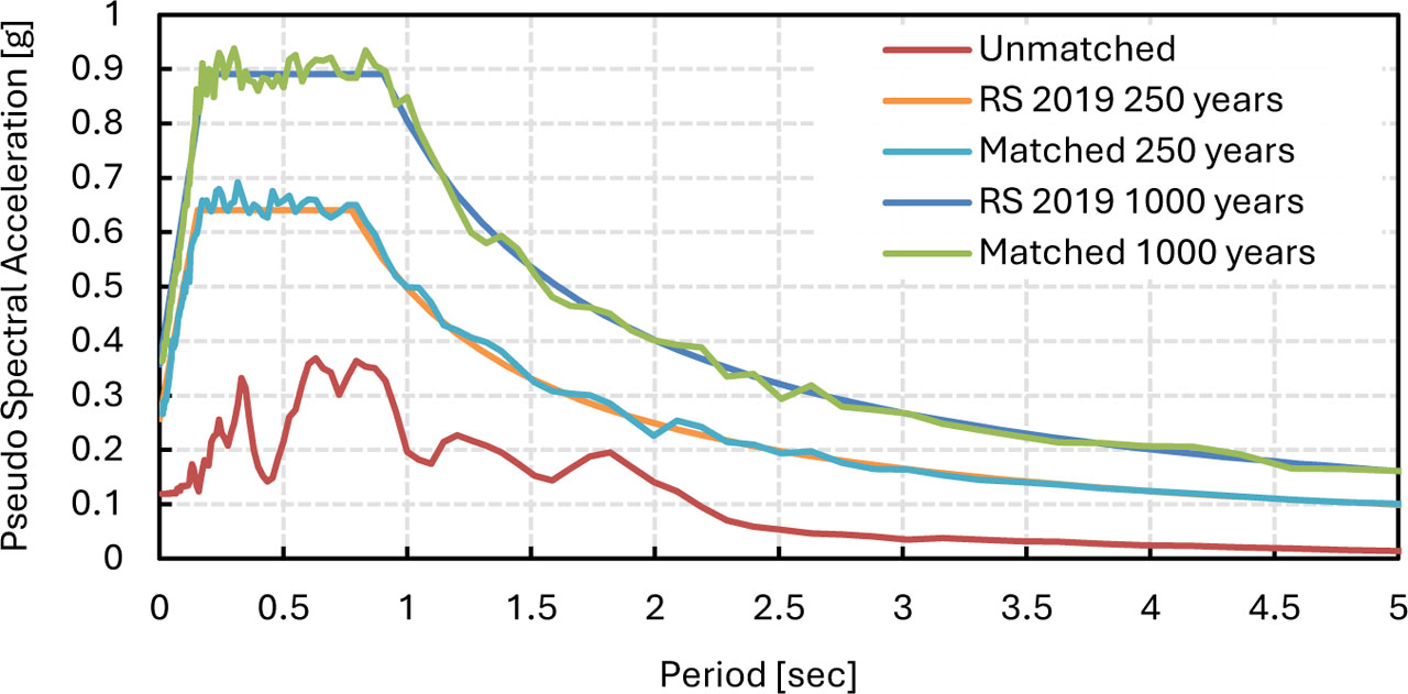
Figure 12:
Spectral response of ground motions Loma Prieta 1989 before and after matching the targeted-site spectral response of earthquake with 250 and 1000 years of return period
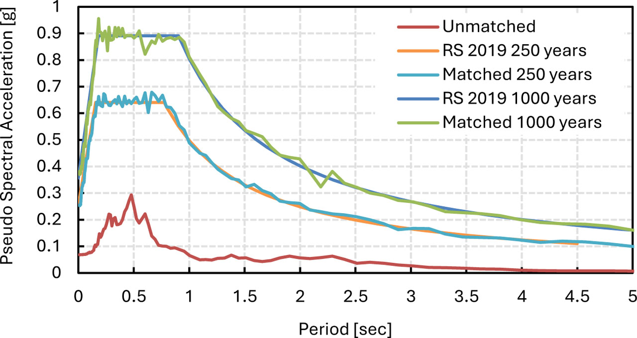
Figure 13:
Spectral response of ground motions Tohoku 2011 before and after matching to the targeted-site spectral response of earthquake with 250 and 1000 years of return period
5. Results of the NLTH Analysis
This study presents the seismic evaluation of an existing building with the addition of a BI protection system. Therefore, as per ASCE 41-17, the existing building should be evaluated against earthquakes with 250 years (BSE-1E) and 1000 years (BSE-2E) of return periods.
5.1. Base Shear
Figure 14 and Figure 15 show the comparison of the average maximum base shear of four models subjected to seven ground motions with 250 (BSE-1E) and 1000 years (BSE-2E) of return periods in X and Y directions. It is shown that in the case of earthquakes BSE-1E, the implementation of the BI system could dramatically reduce the base shear by as much as 46% and 44% in X and Y directions, respectively, which indicates significant protection on the existing building under study. When the SSI effect was considered, remarkable increases in the base shear were observed by as much as 52% and 23% in the X and Y direction, respectively, in the case of the FB model. As expected, the effectiveness of the BI system in reducing the base shear decreased with the presence of SSI. However, when compared to the fixed-base model with the effect of SSI (FB+SSI), a significant reduction in the average base shear was still present.
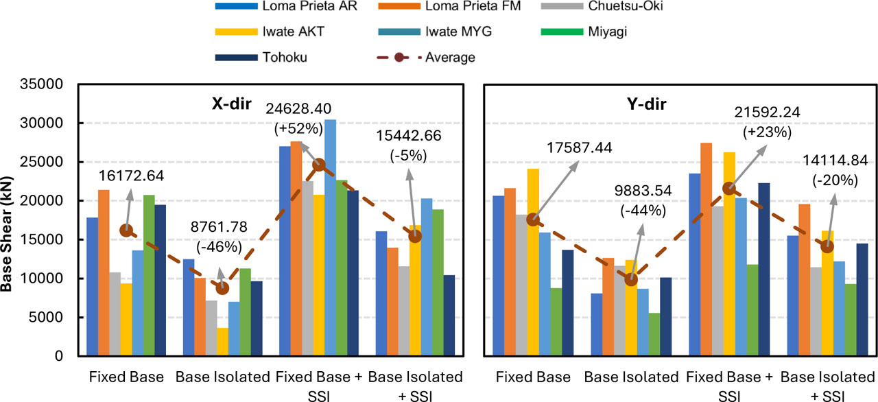
Figure 14:
Comparative charts of the peak base shear in X and Y directions under earthquakes BSE-1E
When larger earthquakes BSE-2E were considered, similar trends of average maximum base shear variation were reported, as seen in Figure 19. The reduction of base shear with the presence of the BI system was almost similar when compared to the case of smaller earthquakes. On the other hand, under the earthquake of 1000 years return period, the effect of SSI on the increase of base shear was smaller. As shown in model FB+SSI, the increase of base shear was observed at only 9% and 8% in the X and Y directions, respectively. Such an increase is much smaller than the increase of base shear due to the SSI effect under BSE-1E earthquake conditions.
In the case of both earthquake levels, it is revealed that the consideration of the SSI effect may lead to a more cautionary design, as presented by the increase of base shear either in fix-based or isolated models. Such an increase might be caused by the amplification due to close values between the fundamental period of the upper structure and the period of the site. However, the effect of SSI was observed much more pronounced in the case of smaller earthquakes.
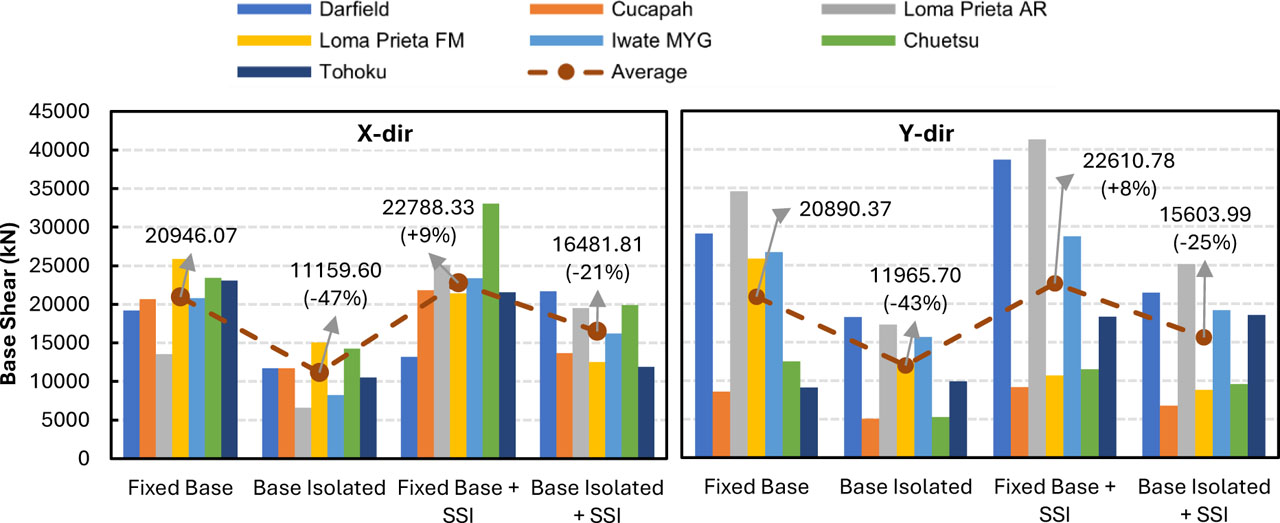
Figure 15:
Comparative charts of the peak base shear in X and Y directions under earthquakes BSE-2E
5.2. Performance of BI System
During the time history analyses, the displacements and forces exhibited by the LRB isolators in the base-isolated models were observed to evaluate whether the capacity of the LRBs was exceeded. The peak lateral displacements obtained from each earthquake were reported in Table 6. The considered lateral displacement was the square root of the sum of the squares of the LRB displacements in the X and Y directions. In the BI model without the SSI effect, the average peak LRB displacements under earthquake levels BSE-1E and BSE-2E were found 119.09 and 213.13 mm, respectively.
The consideration of SSI resulted in more critical behaviour. The average peak lateral displacements of the BI system were found to increase by 9.28% in the case of earthquake BSE-1E and by 6.90% in the case of earthquake BSE-2E. In all cases, the peak lateral displacements of the BI system, as much as 297.74 mm, were reported below the target maximum displacements during the preliminary design of the isolation system.
Table 8:
Peak isolator displacements observed in NLTH analysis
| Parameter | Earthquake event | Base isolated | Base isolated + SSI |
|---|---|---|---|
| Isolator horizontal displacement (mm) 250 yr | Loma Prieta AR | 150.481 | 154.52 |
| Loma Prieta FM | 124.685 | 130.752 | |
| Chuetsu-Oki | 112.451 | 136.797 | |
| Iwate AKT | 70.355 | 77.644 | |
| Iwate MYG | 109.309 | 157.749 | |
| Miyagi | 133.495 | 142.794 | |
| Tohoku | 132.831 | 110.761 | |
| Average | 119.09 | 130.15 (+9.28%) | |
| Isolator horizontal displacement (mm) 1000 yr | Darfield | 279.173 | 297.74 |
| Cucapah | 277.722 | 210.176 | |
| Loma Prieta AR | 265.88 | 270.982 | |
| Loma Prieta FM | 233.222 | 165.959 | |
| Iwate MYG | 167.229 | 217.09 | |
| Chuetsu | 156.097 | 174.313 | |
| Tohoku | 112.558 | 258.589 | |
| Average | 213.13 | 227.84 (+6.90%) |
5.3. Inter Story Drift
The level of structural damage to the building during an earthquake can be identified through the inter-story drift. Figure 16 and Figure 17 present the peak inter-story drift at different floor levels from the NLTH analyses. Under earthquake level BSE-1E, as shown in Figure 16, the presence of the BI system resulted in a considerable positive effect by reducing the average inter-story drift by approximately 19%–24%. Furthermore, a much more pronounced effect of the BI system was observed under the earthquake level BSE-2E where a reduction of average inter-story drift was reported at 49%, approximately, as shown in Figure 17. On the other hand, excessive drifts were observed at the base floor level. However, this issue can be addressed by increasing the lateral stiffness of the floor by increasing the column dimension or adding shear wall or bracing system.
In the other case, when the SSI is considered in the fixed-base model, a remarkable increase in average inter-story drift was observed, as much as 13%–30%, approximately, in the case of earthquake level BSE-1E, as shown in Figure 16. On the other hand, under larger earthquake level, BSE-2E, the effect of SSI in the fixed-base model is much less pronounced as the change of inter-story drift was negligible: as much of −2% to −6%, approximately, as shown in Figure 17.
Regarding the SSI effect in the base-isolated model, slight to negligible effects on the inter-story drift were shown, both under earthquake BSE-1E and BSE-2E. It again indicates that the BI system was able to isolate the effect of SSI on the performance of the structure.
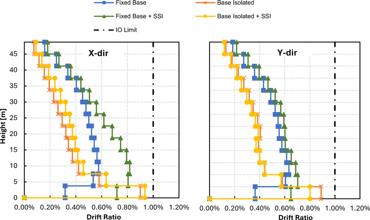
Figure 16:
Maximum interstory drift in X and Y directions under earthquake BSE-1E
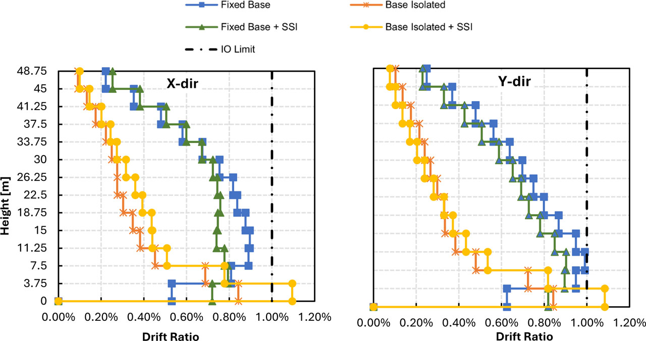
Figure 17:
Maximum interstory drift in X and Y directions under earthquake BSE-2E
5.4. Acceleration Response
The comparison of the acceleration responses in X and Y directions at the top roof level is presented in Figure 18 and Figure 19. At the level of both earthquakes BSE-1E and BSE-2E, the implementation of the BI system was found effective in significantly reducing the acceleration response by approximately 43–48%. This remarkable reduction of acceleration response may promote the utilization of the BI system to ensure the comfort of building occupants and avoid damage to non-structural components or sensitive devices during earthquakes, regardless of the soil conditions.
Regarding the effect of SSI modelling, both in fixed and isolated models, the consideration of SSI presented a slight or negligible effect on the acceleration response of the upper structure, both in the case of small and large earthquakes.
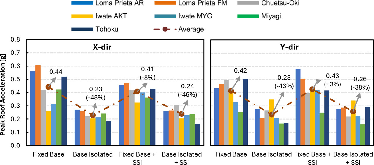
Figure 18:
Comparative charts of peak acceleration response at the roof level in X and Y direction under earthquakes BSE-1E
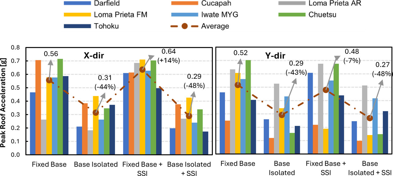
Figure 19:
Comparative charts of peak acceleration response at the roof level in X and Y direction under earthquakes BSE-2E
6. Comparison to Previous Studies
To validate and contextualize the findings of this study, a comparison with previous research on soil–structure interaction (SSI) is conducted. The results obtained in this study are consistent with those reported by Karabork et al. (2014) and Mohasseb et al. (2019), where the inclusion of SSI leads to a significant amplification of structural responses. In Karabork et al. (2014), SSI resulted in increases in base shear (+190%), roof acceleration (+168%), natural period (+137%), and roof displacement (+44%), indicating a substantial increase in system flexibility. Similarly, Mohasseb et al. (2019) reported that SSI increases the natural period by approximately +42% and roof displacement by approximately +77% to +112%, further confirming that SSI introduces additional flexibility into the soil–foundation system and amplifies deformation demand.
In contrast, Yanik and Ulus (2023) observed a different trend, where SSI increases the structural period by approximately +8.5%, while reducing roof displacement by approximately −50% and roof acceleration by approximately −73%. This behaviour reflects a trade-off mechanism associated with period elongation, in which the structural response shifts toward a lower spectral acceleration region, resulting in reduced force demand but increased displacement demand of the building.
Overall, the comparison indicates that SSI consistently increases structural flexibility (approximately +8.5% to +137% in period), while its influence on structural responses such as displacement and acceleration may vary depending on system characteristics. The results of this study fall within this range of behaviour, thereby reinforcing the importance of explicitly considering SSI effects in the seismic analysis and design of base-isolated structures.
7. Conclusion
A series of nonlinear time-history analyses were conducted to evaluate the effectiveness of a lead–rubber bearing (LRB) base isolation (BI) system for seismic protection of a 13-story existing MRF-RC building founded on soft soil, explicitly considering soil–structure interaction (SSI) through an indirect modelling approach using translational springs. Ground motions representing 250-year (BSE-1E) and 1000-year (BSE-2E) return periods were applied, and multiple seismic performance parameters were assessed. Based on the obtained results, several conclusions can be drawn:
▪ The BI system significantly lengthened the fundamental period of the structure from 1.801 s to 3.857 s in the fixed-base (FB) condition, while SSI slightly increased structural flexibility in both FB and BI models.
▪ BI enhanced the cumulative modal mass ratio (CMMR) in the lower vibration modes, improving dynamic response, although SSI reduced the CMMR in all cases.
▪ Base shear was reduced by up to 46% (BSE-1E) and 47% (BSE-2E) with BI compared to the FB model, while SSI tended to increase base shear – especially under BSE-1E.
▪ Peak floor acceleration was decreased by approximately 48% with BI at both earthquake levels, while SSI had minimal influence on acceleration response.
Overall, the results highlight that SSI can have a detrimental impact on the seismic performance of fixed-base structures on soft soil, and advanced SSI modelling is essential in such cases. However, the implementation of the BI system not only improved overall seismic performance but also significantly mitigated the negative effects of SSI, particularly in terms of plastic hinge formation and inter-story drift, further reinforcing its applicability for high-rise buildings on soft soil sites.
Acknowledgements
The authors would like to acknowledge the financial support to perform the research from the Indonesian National Research and Innovation Agency (BRIN) with grant number 1179/PKTS/ITS/2023 (RIIM Program).
Notes
[1] Contributed by Author Contributions
M.F.F. prepared the initial draft of the manuscript and performed the software development and simulations together with F.F.; A.B.H. and N.K. contributed to funding acquisition and methodology, in collaboration with G.P.; F.F. and G.M. supervised the overall research process; G.P. and G.M. provided critical review and improvements to the writing. All authors read and approved the final manuscript.