

1. Introduction
In recent years, the application of carbon fiber reinforced polymer (CFRP) for strengthening ultra-high-performance concrete (UHPC) has gained significant attention due to UHPC’s superior mechanical properties and dense matrix, which enhance the bond performance with CFRP. Finite element (FE) analysis has become a critical tool for understanding and predicting the structural behavior of CFRP-strengthened UHPC elements. For instance, (Abbas et al. 2020) developed a 3D nonlinear FE model to simulate the flexural performance of CFRP-strengthened UHPC beams and found good agreement with experimental results, highlighting the accuracy of FE simulations in capturing failure modes and load-displacement responses. Similarly, (He et al. 2019) conducted a numerical investigation using ABAQUS and demonstrated that the interfacial bond between CFRP and UHPC plays a crucial role in controlling debonding failure, emphasizing the need for accurate bond-slip modeling. (Moreover, Ma et al. 2021) introduced a cohesive zone model to simulate the interface behavior between CFRP and UHPC, which effectively predicted delamination patterns under shear loading. These studies underline the effectiveness of FE modeling in optimizing CFRP retrofit strategies and contribute to a better understanding of the structural behavior of UHPC composites. However, further research is still needed to calibrate interface models and validate them across different strengthening configurations and load scenarios.
Furthermore, most past studies either focus on flexural strengthening or small-scale bond tests, with insufficient attention to shear-critical regions and the role of CFRP in shear retrofitting of UHPC members. To address this gap, our study proposes FE models and an experimental program involving full-scale UHPC beams retrofitted with externally bonded CFRP sheets, aiming to assess their shear performance. The novelty lies in both the scale of testing and the targeted behavior (shear).
“(Dewi et al. 2024) conducted experimental tests on hollow circular RC columns strengthened with CFRP strips and validated a finite element (fiber element) model which closely matched the experimental strain results across reinforcement and CFRP layers. This confirms the reliability of FE modeling for predicting behavior of CFRP-strengthened concrete elements.”
“In (Maulana et al. 2025), finite element analysis was used to simulate CFRP-strengthened beam-column joints, showing that extending CFRP sheets to twice the beam height significantly improves seismic and shear resistance. Another study (CEE, 2025) performed numerical FE modeling on composite-strip-strengthened concrete beams, validating the reliability of the FE approach for predicting structural improvements comparable to CFRP strengthening.”
This paper contains a description of reinforced concrete beams that were strengthened using the CFRP sheets technique by experimental methods employing FE models. To compare the experimental results, the simulation was conducted in ABAQUS 6.14 under monotonic two-point loading. The Concrete Damaged Plasticity model was applied to simulate the irregular behavior of concrete, and its properties were derived from the results of experimental tests. The model contained both unimproved and strengthened CFRP beams to understand shear behaviour and check the success of strengthening the beams. Major aspects of bar interaction were described to make sure the simulation was accurate. The objective of the developed model was to imitate the ways failures and cracks spread in the material during the tests.
2. Description of the Test Specimens used in validation
All specimens had beams of the same geometry and concrete grade, resulting in equal compressive strength in all cases (Concrete mix information and details are listed in Table 1. The choices for shear reinforcement in the beams differed a lot. In the control specimen, known as RC-C Beam, there was a tiny internal reinforcement to resist shear, with only two shear links added close to the supports and without external CFRP treatment.
Table 1:
Concrete mixes
| Mixes all in [kg/m3] | Fine sand | cement | Water | Superplastizer | Silica Fume | Fly Ash | Compressive strength [MPa] 28 days |
| 1070 | 970 | 184 | 33.4 | 107 | 192.6 | 126.97 |
Different types of CFRP reinforcement were used on the other beams to find out which was best. This specimen, RC-CFRP-U-90-100 Beam, included U-shaped CFRP strips joined with epoxy and arranged perpendicular (90 degrees) to the beam axis from the beam’s center support to the load point. These strips were spaced 150 mm apart center-to-center. A similar beam, the RC-CFRP-U-45-100, used the same width and spacing of CFRP strips but oriented at a 45-degree angle, offering a different shear reinforcement configuration. Another design, the RC-CFRP-2SIDE-600 Beam, employed wide (600 mm) epoxy-bonded CFRP strips applied to both sides of the beam, again extending from the center point of the support to the load point. The RC-CFRP-U-90-600 Beam followed a similar pattern but with U-shaped strips at a 90-degree angle on each side. Lastly, the RC-CFRP-FULL FACE Beam utilized full-face epoxy-bonded CFRP strips, also 600 mm wide, covering the entire side surfaces between the support and load center to maximize shear strengthening.
All beams were uniformly dimensioned at 200 mm width, 400 mm depth, and 2050 mm length as illustrated in Figure 1. The testing setup involved simply supported specimens subjected to four bending points, with supports placed 125 mm from the beam ends, according to ASTM C1609 or general practices in shear and flexural testing of concrete. The loading was load-controlled and monotonically applied at a constant rate of two kN/min. Reinforcement included three 16 mm diameter deformed steel bars at the bottom and two at the top, maintaining a longitudinal steel ratio of 1.67% in both layers. This flexural reinforcement was intentionally designed to prevent flexural failure, allowing the study to focus solely on the shear resistance provided by the CFRP strengthening. The effective depth was measured at 367 mm, with a concrete cover of 25 mm, ensuring consistent protection for the steel bars.
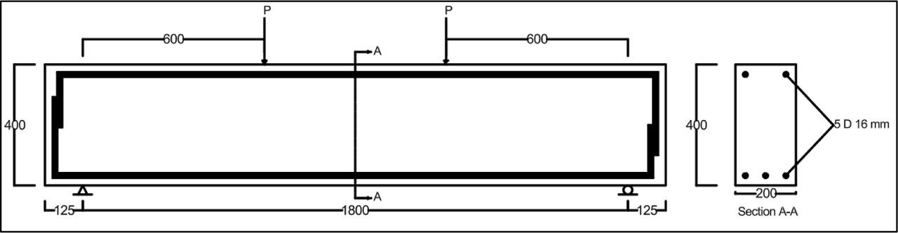
Figure 1:
Dimension and reinforcement details of specimens (all dimensions in mm)
3. CFRP Reinforcement Configuration
In this study, CFRP was employed in various shear strengthening arrangements, as outlined in Table 2. The first beam, serving as a control specimen, was tested without CFRP reinforcement, as shown in Figure 2. The CFRP strips employed for shear strengthening were 100 mm wide and spaced at 150 mm center-to-center. The length of each strip corresponded to the full depth of the beam (400 mm) and was adjusted accordingly when applied at angles other than 90°, to account for the increased length resulting from the inclination.
In one configuration, the strips were oriented at 90 degrees, as illustrated in Figure 3, while in another, they were placed at a 45-degree angle, as shown in Figure 4. For the two-sided strengthening scheme, wider CFRP strips measuring 600 mm in width were bonded to both sides of the beam, as shown in Figure 5. The U-shaped configuration featured 600 mm-wide CFRP strips attached to the tension face at the bottom and to both side faces, as seen in Figure 6. Similarly, a closed-shaped arrangement involved wrapping CFRP strips around all faces of the beam, as illustrated in Figure 7. CFRP sheets were installed along the shear span, starting from the points of support to the locations where the loads were applied on both sides
Table 2:
CFRP-Reinforcement Configurations and Strengthening
| Sample | CFRP strengthening type at each side | Cfrp orientation [degrees] |
|---|---|---|
| RC-C | Without | / |
| RC-U-90-100 | U- shape,100 mm width,150mm spacing c/c | 90° |
| RC-U-45-100 | U- shape,100 mm width,150mm spacing c/c | 45° |
| RC-2side-90-600 | 2-sided-shape,600 mm width | 90° |
| RC-U-90-600 | U- shape,600 mm width | 90° |
| RC-Full-Face | Full Face | 90° |
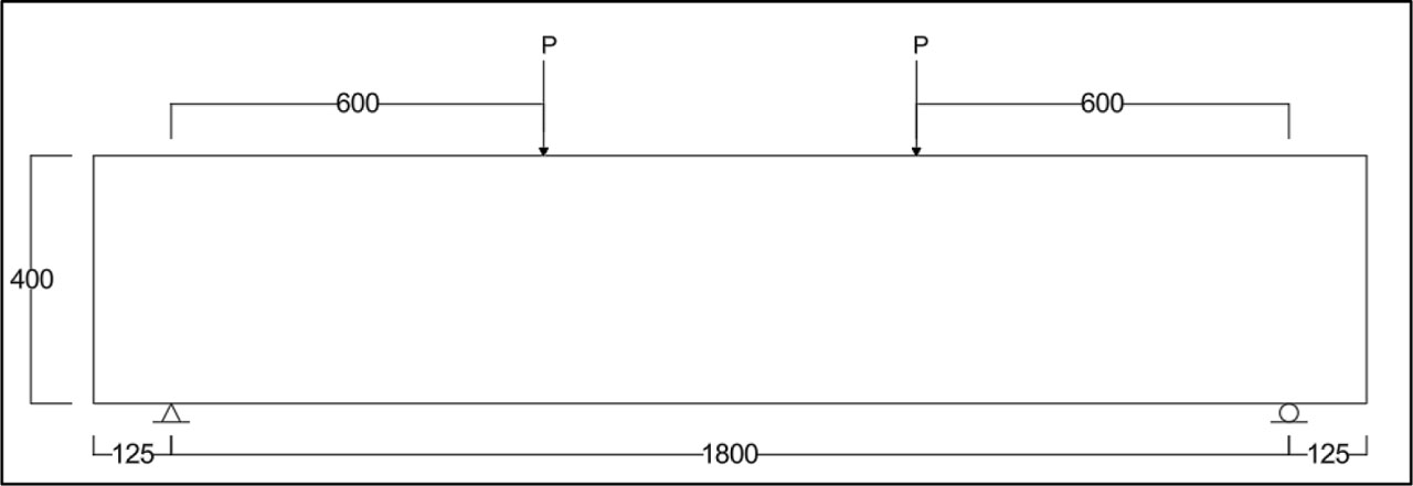
Figure 2:
(RC-C) control specimen (all dimensions in mm)
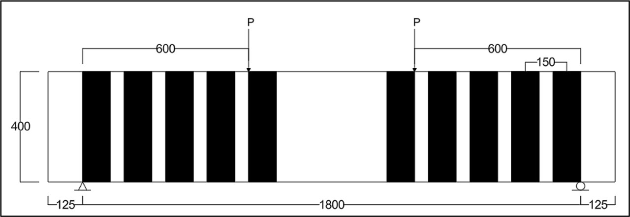
Figure 3:
(RC-CFRP-U-90-100) (all dimensions in mm)
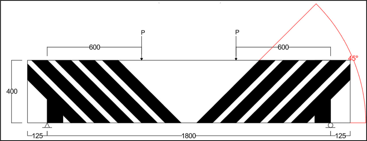
Figure 4:
(RC-CFRP-U-45-100) (all dimensions in mm)
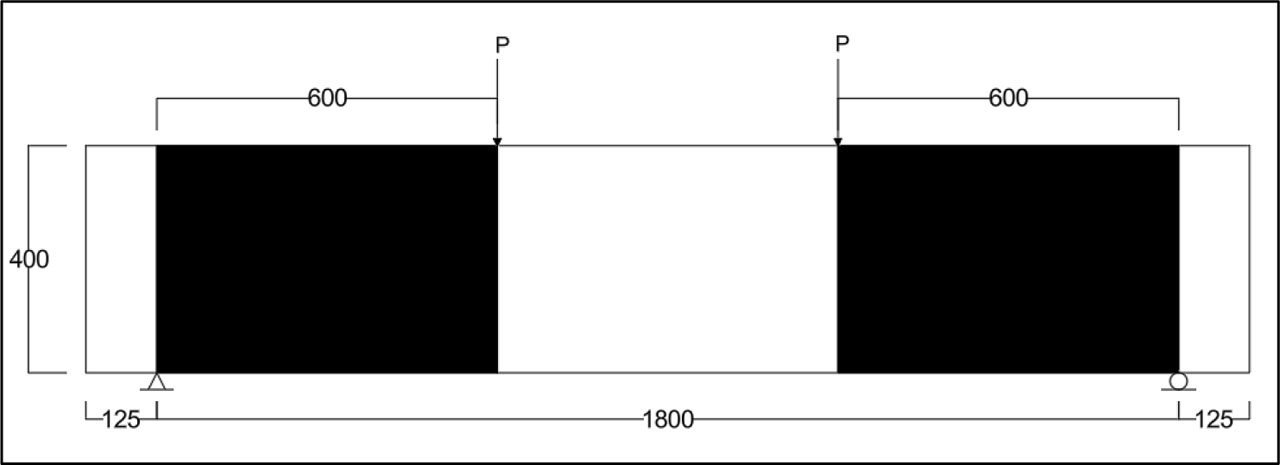
Figure 5:
(RC-CFRP-2side-90-600) (all dimensions in mm)
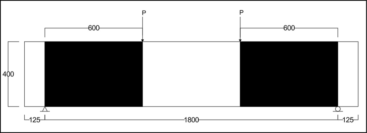
Figure 6:
(RC-CFRP-U-90-600) (all dimensions in mm)
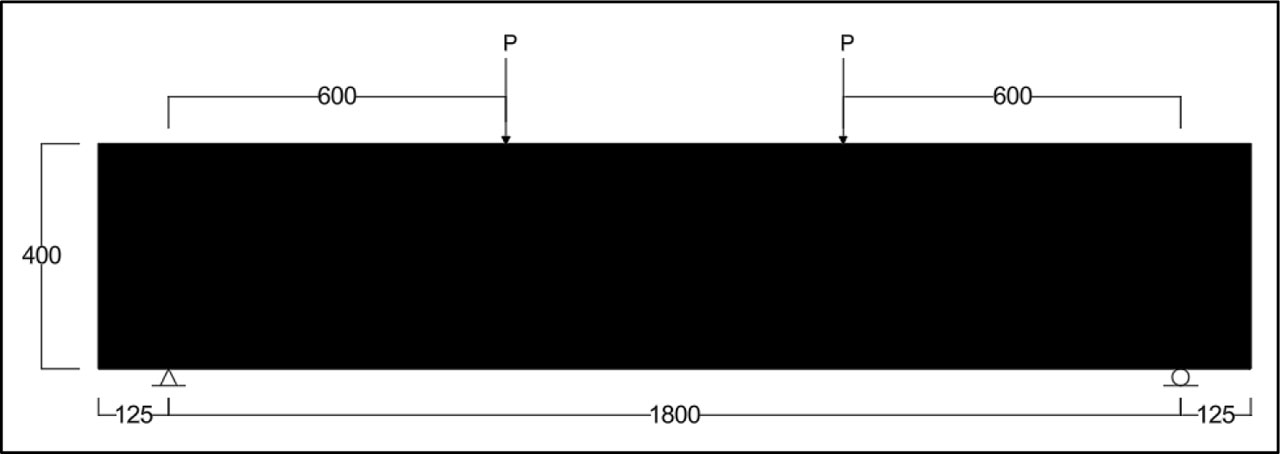
Figure 7:
(RC-CFRP-Full Face) (all dimensions in mm)
4. Definitions
The major parts of the reinforced concrete beams are the concrete, steel reinforcement inside, and CFRP sheets added for shear strength. Each part of the analysis should capture the actual behaviour of the materials in monotonic stressed RC beams strengthened with CFRP. Material models available in the ABAQUS library reflect how every physical component behaves.
4.1. Material Modelling
4.1.1. Steel Reinforcement
You can use ABAQUS to include reinforcement using smeared reinforcement in the concrete mass, explicit truss or beam elements together with an embedded region constraint, or predefined layers of rebar. Rebar sets the reinforcement for membrane, shell and surface elements in terms of uniaxial reinforcement. The user must set up one or more options for reinforcing the behavior. For every layer, they should choose a label for the rebar layer, set the cross-sectional area per layer, and determine how far apart the rebars are arranged in the mentioned direction. This comes from their study (Malm, R., & Ansell, A. 2009). This part of the report will only cover embedded region modelling, which was used for reinforcement modelling in the study. To use the truss method, you just need to enter the area of the reinforcement bars. Another popular tactic for structures is to use beam element modelling, which recognizes the dowel effect and slightly makes the structure stronger. On the other hand, using this approach is not suggested since defining a large amount of input parameters takes a lot of computing power (Eriksson, D., & Gasch, T. 2011), (Hibbitt, Karlsson & Sorensen, Inc. 2014), and (Malm, R. 2009). (Hibbitt, H., Karlsson, B., & Sorensen, P. 2011) Writers state that bond slip is not included in the implementation of embedded region modelling. Still, the stiffening effect of concrete, according to (Malm, R. 2009), includes some of these aspects.
4.1.2. Concrete
Smeared cracking and concrete damaged plasticity (CDP) are the two techniques available in ABAQUS for describing the actions of concrete. The smeared cracking model deals with beams, trusses, solids, and shells. This type of inquiry does not pay attention to each minuscule crack in the system. The CDP was introduced by applying the yield function from the paper written by (Lubliner, J., Oliver, J., Oller, S., & Onate, E. 1989). Here, linear elasticity gives a true account of how materials act under compression as well as tension. Tensile cracking and compression fractures are the two ways the model may fail. The CDP model is very popular as it accurately depicts the actions of concrete. For calculations involving non-straight forces in concrete, it is especially effective because it gives a thorough account of the material’s behaviour (especially in reinforced concrete members affected by shear) (Tyau, J. S. 2009).
Principle of concrete damaged plasticity formulation
Two important things define the damaged plasticity model: decreasing properties under compression and tension. Changing the initial stiffness of the member permits the element’s elastic stiffness to decrease when it goes into plasticization.
Where:
The subscripts t and c refer to tension and compression, respectively.
, and , These are the equivalent plastic strains.
θ is the temperature.
fi - (i = 1,2,3,4,...) are other predefined field variables (Hibbitt, H., Karlsson, B., & Sorensen, P. 2011).
The numbers for “damage parameters” go from zero for undamaged and unchanged material to one for destroyed material. You can find the effects of the plasticity default in Figure (8). As you see in Figure (8), the curve shows the stress versus strain for tension and compression. A dotted line shows the shape of the curve. The purple line represents the shape of cyclic loading that happens when the element is in severe damage, and it experiences tension past its tensile strength limit. Reveal that communities often use colour to form their identities. Yet only part of the material is damaged in cracking, and this can be denoted by the amount of time dt. You can determine the elastic behavior after unloading by multiplying the original modulus by (1 – dt). Parameter wc shows the percentage of change in stress due to strain, and the compression modulus is given by (1 − dt + wc dt) (Colavita, M. M., Serabyn, E., Millan-Gabet, R., Koresko, C. D., Akeson, R. L., Booth, A. J., Mennesson, B. P., Ragland, S. D., Appleby, E. C., & Berkey, B. C. 2009).
You should also notice that when a crack appears, compression stiffness does not change, so wc is still constant at one. If the stiffness brought by complete destruction and compression does not change with tension, the parameter (wc) will equal zero. The attributes lost in the bashing part are shown by the dc variable, while wt represents the initial status in tension.
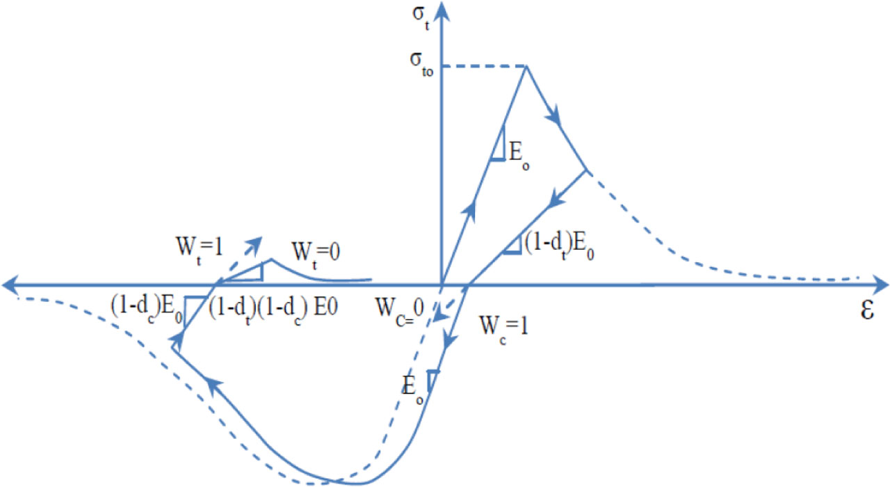
Figure 8:
Uniaxial load cycle (tension-compression-tension) ABAQUS 6.14
Concrete Plasticity Parameters
The adjustments given can be implemented to calculate the flow potential yield surface, first introduced by five important factors that need to be established to achieve this. Having tested many different materials, specialists could better determine the values of these parameters. However, all the default settings in ABAQUS were applied (Lubliner, J., Oliver, J., Oller, S., & Onate, E. 1989) and (Lee, J., & Fenves, G. L. 1998).
The five parameters that need to be defined are:
∈: When approaching the asymptote, Drucker-Prager function uses the rate ∈ to describe the curve. If eccentricity goes towards zero, the plastic stream moves towards a straight line. In the next steps of computation, the eccentricity was assumed to be 0.1. It allows a mild curvature in the potential flow and about the same dilation angle across a variety of confining pressure values, as is demonstrated in (9).
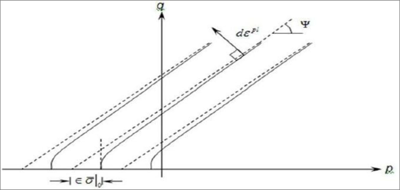
Figure 9:
Flow potentials in the p-q plane CAE (Hibbitt, H., Karlsson, B., & Sorensen, P. 2011)
Integer “∈bo/∈co” Parameter: That is the initial unidirectional compressive strength compared to the equiaxial compressive strength ratio. It is vital to determine the yield function. Figure (10) illustrates that we have used 1.16 as the initial constant, the default patient default risk.
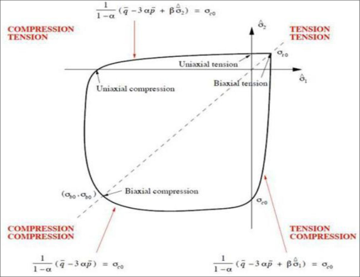
Figure 10:
Yield surface in plane stress (Yu, J., Chen, S., Li, L., & Wang, H. 2011)
μ: stands for the parameter related to viscosity. It must be addressed when the problem arises due to decreasing stiffness of plastic and elastic materials. It’s easier for flat-plate models to converge for the μ value of 0.000375, thus this value gives the best results. If the parameter of viscosity equals zero, the material turns plastic, and divergence happens directly after the crack forms. The solution stretches out if μ is large in comparison to the time increment step. Generally, making the viscosity parameter small will improve the solution without affecting the outcome. The paper says that μ should be set to 15 percent of the time increment step (Lee, J., & Fenves, G. L. 1998).
Ѱ: dilation angle is the descriptor of the rate of change between volume and shear strain, found in the p – q plane at high confining pressure where p = − 1/3 (2σ1+ σ3) and indicate hydrostatic pressure stress and Misses equivalent effective stress respectively and σ1 σ3 stand for the highest and lowest principal stresses in a triaxle test. Virtually all the published data used dilation angles for concrete that vary between 12° and 37° (Hibbitt, H., Karlsson, B., & Sorensen, P. 2011) and (Ennochsson, O., Lundqvist, J., Täljsten, B., Rusinowski, P., & Olofsson, T. 2007).
Kc: means the ratio between the second stress invariant on T.M. and C.M., and it is a ratio used to describe the yield surface in a deviatoric plane depicted in Figure (11), and it should always be within the range 0.5 ≤ Kc ≤ 1.0.
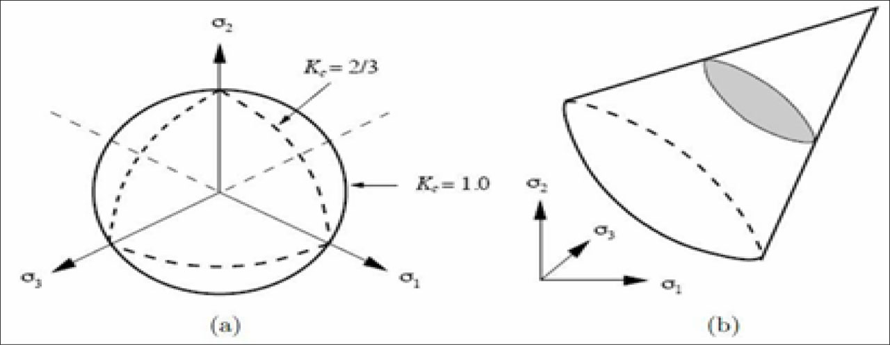
Figure 11:
(a) Drucker-Prager Yield Criteria in the Deviatoric Plane for Different Kc (Hibbitt, H., Karlsson, B., & Sorensen, P. 2011) and (b) Yield Surface in 3D for Kc =1 (Pankaj, P. & Donaldson, C. 2013)
Concrete Tensile Behaviour
ABAQUS standard supports three different methods to define the way post-cracking tension reduces. The methods are to specify strain, crack opening (displacement), or fracture energy, as shown in Figure (12). Plain concrete’s sensitivity to fine mesh can be seen by the strong influence of tensile stress and strain on the strength criterion. The predicted results keep varying as the mesh is refined. As a result, more mesh points make the cracks narrow, but there are fewer new fractures. Hence, you shouldn’t rely on the strain technique for components without reinforcing, as the structure often collapses spots. Yield stress-cracking strain data represent the process of softening data. Calculating cracking strain means taking the overall strain and then subtracting out the strain the undamaged material would experience. Mathematically, it may be expressed as where . This relationship is illustrated in Figure (12) (a).
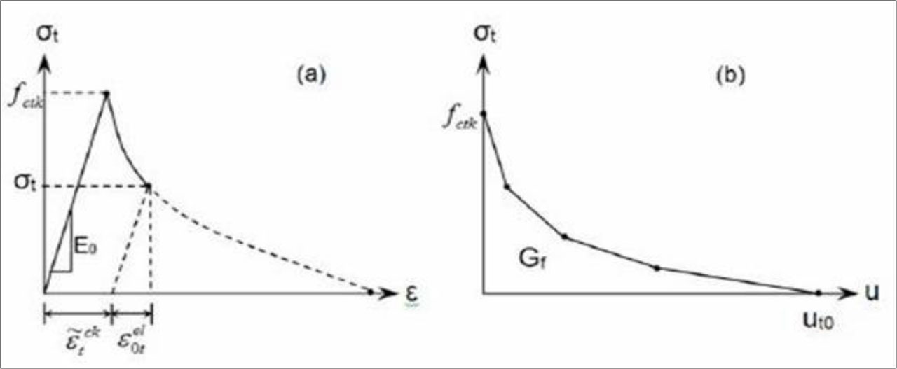
Figure 12:
(a) post-failure tensile behaviour:(a) stress-strain approach;(b) fracture (Hillerborg, A., Modéer, M., & Petersson, P.-E. 1976)
Alternatively, fracture energy and stress displacement can collectively be used to describe the tensile behaviour of concrete as they relate to cracking. They both use a cracking criterion devised by (Hillerborg, A., Modéer, M., & Petersson, P.-E. 1976), which eases the disadvantage of the older method caused by mesh dependence. The stiffness of concrete, which is a brittle behaviour, is shown by a tensile stress-displacement
The strategy depends on the concepts of brittle crack theory. Gf stands for concrete fracture energy and is the energy used to create a crack with a given area. Basically, fracture energy means the energy that results from the area under the tensile load curve and displacement for fracture.
Tension Stiffening Model
As the fractured concrete meets the steel, the tensile load it takes is normal to the crack, creating the rigidity strengthening of the concrete. To reach this, the stress component in the concrete is gradually released on the plane that goes across the crack. In the current analysis, three ways of representing the models using strength conditions were chosen: linear, bilinear, and exponential curves. Figure (13) represents the results from the research that was performed (Hsu, H.-M., & Wang, W.-P., 2001). (Bažant, Z. P., & Oh, B. H., 1983) worked with Oh to produce the bilinear curve.
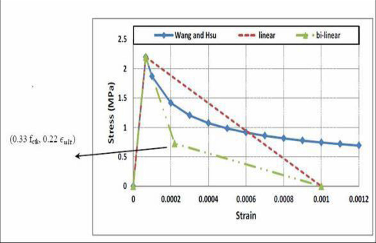
Figure 13:
Uniaxial tensile stress-strain behavior of concrete (Hsu, H.-M., & Wang, W.-P. 2001)
Concrete Compressive Behaviour
Concrete exhibits linear elastic behavior up to about 30–40% of its ultimate compressive strength. Beyond this range, microcracking initiates, and the material behavior becomes nonlinear. Therefore, the presence of cracks in the primary structure indicates that the concrete has exceeded its elastic limit and entered the nonlinear phase, which affects its load-carrying capacity. This behavior is well documented by (Neville 2011), who explains the transition from elastic to nonlinear behavior in concrete under compression. Additionally, (Mander, Priestley, and Park 1988) provide a theoretical stress-strain model for confined concrete that captures this nonlinear response. ABAQUS states that the level of hardening and strain softening is linked to the compressive stress and the elastic strain, so their connection is shown by the equation
Where:
ɛ0cel = σc / Ecm and Ecm It is the initial modulus of elasticity.
The model was proposed by (British Standards Institution. 2004). Eurocode 2 brings together several rules and recommendations on how concrete in Europe should be built. The modelling methods and the design details in this case are discussed with finite element analysis.
You should remember that the terms in equation (5) are correct only if 0 < |ɛc1| < |ɛcu1|. The nominal ultimate strain is represented by ɛcu1, and its value is about 0.0035. At the highest point of tension, strain is ɛc1 as shown in Table 3. The word fcm is used to show compressive strength.
Table 3:
Strength and deformation characteristics of concrete (British Standards Institution, 2004)
| Strength classes for concrete | Analytical relations / Explanation | ||||||||||||||
|---|---|---|---|---|---|---|---|---|---|---|---|---|---|---|---|
| fck (MPa) | 12 | 16 | 20 | 25 | 30 | 35 | 40 | 45 | 50 | 55 | 60 | 70 | 80 | 90 | |
| fck,cube (MPa) | 15 | 20 | 25 | 30 | 37 | 45 | 50 | 55 | 60 | 67 | 75 | 85 | 95 | 105 | |
| fcm (MPa) | 20 | 24 | 28 | 33 | 38 | 43 | 48 | 53 | 58 | 63 | 68 | 78 | 88 | 98 | fcm = fck + 8 (MPa) |
| fctm (MPa) | 1,6 | 1,9 | 2,2 | 2,6 | 2,9 | 3,2 | 3,5 | 3,8 | 4,1 | 4,2 | 4,4 | 4,6 | 4,8 | 5,0 | |
| fctk,0,05 (MPa) | 1,1 | 1,3 | 1,5 | 1,8 | 2,0 | 2,2 | 2,5 | 2,7 | 2,9 | 3,0 | 3,1 | 3,2 | 3,4 | 3,5 | fctk,0,05 = 0,7 × fctm 5% fractile |
| fctk,0,95 (MPa) | 2,0 | 2,5 | 2,9 | 3,3 | 3,8 | 4,2 | 4,6 | 4,9 | 5,3 | 5,5 | 5,7 | 6,0 | 6,3 | 6,6 | fctk,0,95 = 1,3 × fctm 95% fractile |
| Ecm (GPa) | 27 | 29 | 30 | 31 | 33 | 34 | 35 | 36 | 37 | 38 | 39 | 41 | 42 | 44 | |
| εc1 (%0) | 1,8 | 1,9 | 2,0 | 2,1 | 2,2 | 2,25 | 2,3 | 2,4 | 2,45 | 2,5 | 2,6 | 2,7 | 2,8 | 2,8 | |
| εcu1 (%0) | 3,5 | 3,2 | 3,0 | 2,8 | 2,8 | 2,8 | |||||||||
4.1.3. Carbon Fiber Reinforced Polymer (CFRP Sheet)
The CFRP composite plate model was treated as an orthotropic material. It behaves in a straight fashion until it can’t handle more stress. The equation below explains the connection between stress and strain in CFRP.
Where:
D1111 to D2323 - Component of the reduced stiffness matrix.
E1 to E3 - Young’s (elastic) modulus in the main material direction 1; 2 and 3.
G12, G13 a G23 - Shear modulus in the 1–2 plane, 1-3 a 2-3.
ν12 - Poisson’s ratio (strain in direction 2 due to stress in direction 1).
ν21- Poisson’s ratio (strain in direction 1 due to stress in direction 2).
ν13 - Poisson’s ratio (strain in direction 3 due to stress in direction 1).
ν31 - Poisson’s ratio (strain in direction 1 due to stress in direction 3).
ν23 - Poisson’s ratio (strain in direction 3 due to stress in direction 2).
ν32 - Poisson’s ratio (strain in direction 2 due to stress in direction 3).
The values of all the variables are presented in Table 4.
Table 4:
Mechanical properties of CFRP sheet (Sika Wrap®-300C) used in Abaqus modelling
| Property | Value [MPa] | Notes |
|---|---|---|
| E1 | 230,000 | Longitudinal modulus (fiber direction) |
| E2 | 16,000 | Transverse modulus (in-plane, epoxy dominated) |
| E3 | 16,000 | Transverse modulus (through-thickness) |
| G12 | 6,894 | In-plane shear modulus |
| G13 | 6,894 | Shear modulus (fiber–thickness plane) |
| G23 | 4,137 | Shear modulus (transverse plane) |
| ν12 | 0.30 | Poisson’s ratio (longitudinal transverse) |
| ν13 | 0.25 | Poisson’s ratio (longitudinal–through-thickness) |
| ν23 | 0.25 | Poisson’s ratio (transverse–through-thickness) |
4.2. Main Meshing Elements
ABAQUS was used to make the simulation model. Two kinds of elements (solid and truss) are used to define various geometric forms. The model in figure (14) includes a mesh.
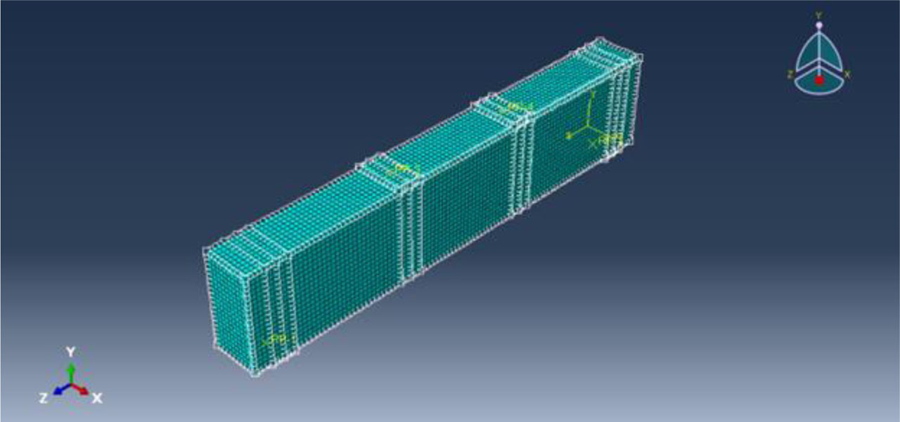
Figure 14:
Mesh for Abaqus model
4.2.1. Solid Element
The design of the concrete part and loading, and B.C pleats were determined in the ABAQUS simulation of the solid part. It took advantage of a 3D element that consists of eight nodes and is linearly reduced. Customarily, quadratic loads placed on slaves in Q4D8R would be applied to the grid; however, with C3D8R we are permitted to use linear brick elements in contact to make concrete parts. Shear locking problems were reduced by adopting the segmented layout instead of the completely merged layout, which looks like Figure (15). It has much in common with actual structure because this method calls for four integration points, adding no shear stress. Integration lines on both sides meet at right angles and the mesh is small.
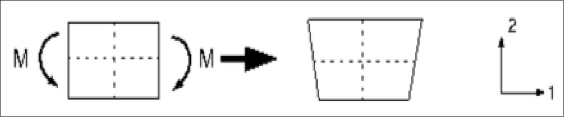
Figure 15:
Linear brick elements undergo pure bending (reduced integration) (Daud, R., Cunningham, L., & Wang, Y. 2015)
4.2.2. Truss Element
The linear three-dimensional model in ABAQUS/Standard (called T3D2) with a two-node truss element and three freedom’s degrees at each node was used to determine the special reinforcing rods in the beam. Figure (16) illustrates that truss pieces are inserted into the 3-D continuum elements acting like a host for the structure. In this analysis, areas called embedded areas represented steel and CFRP. Entering just the cross-sectional area of the bars into a truss element is the best way to reinforce the design. Another popular approach includes beam element modeling that includes the role of dowels and boosts the ability of a structure to hold heavy loads. Even so, it has to be used since it requires setting numerous input values.
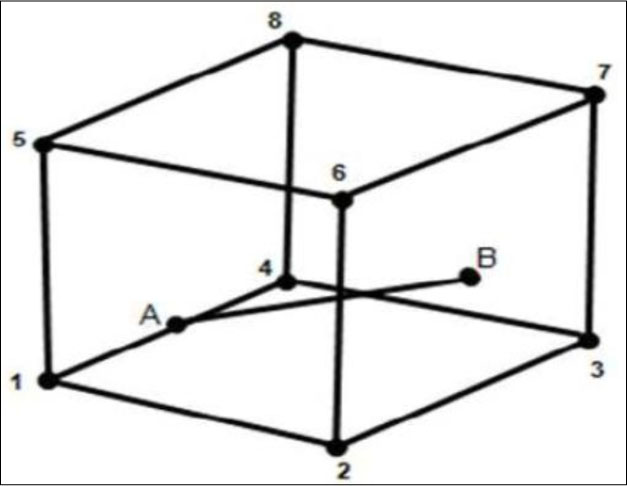
Figure 16:
Element AB is Embedded in (3-D) Continuum Element; Node A is Constrained to edge (1-4), and Node B is constrained to face (2-6-7-3) (Daud, R., Cunningham, L., & Wang, Y. 2015)
4.3. Boundary Conditions
Getting the boundary conditions right was an important element in the finite element modelling done with ABAQUS. It was assumed that the beam’s left side was gently supported, and the right side was free of support, fixed only in the Y direction. So that the model would resemble real conditions, two rectangular support plates (25 × 25 × 200 mm) were placed below both ends. The tie constraint linked the support plates together with the concrete. Support configuration and the boundary conditions are illustrated in Figure (17).
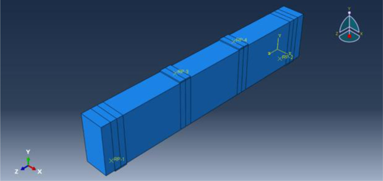
Figure 17:
Boundary Conditions for Beam Model in ABAQUS
4.4. Loads
A monotonic load was applied to the beam in ABAQUS by running the Static General procedure. Loading forced the steel beam by applying pressure on the top of rectangular plates positioned at two spots along the beam’s top surface. Every loading plate measured 25 × 25 × 200 mm, according to the setup used for the experiment. A 25 mm wide assessment of concrete was used to mimic the line load in the real test. The tie constraint was applied to join the load plates to the concrete, so that the pressure is spread smoothly without sliding. As presented in Figure (18), the pressure loads were applied to the model according to a particular setup.
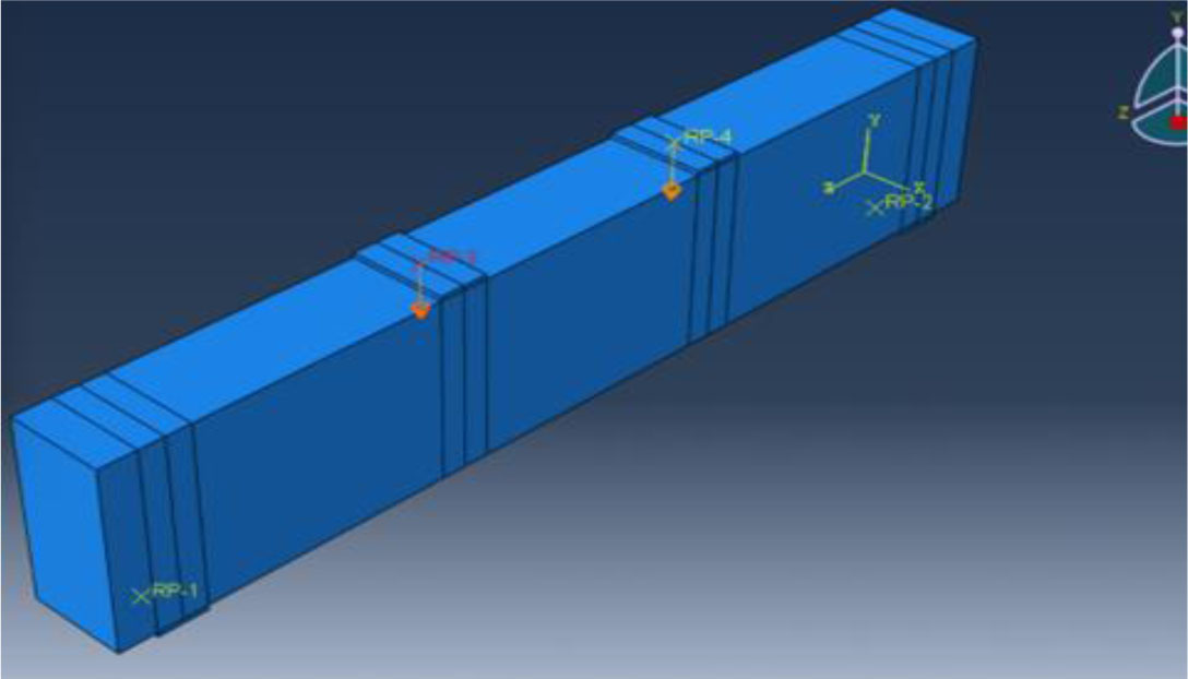
Figure 18:
Specification of Loading Line as Pressure on Beams in ABAQUS
5. Solution Control Parameters
ABAQUS’s Static General procedure was used to carry out the nonlinear finite element analysis. It employed the Modified Newton-Raphson method, which means the stiffness matrix got updated at each iteration to make the convergence faster in cases where the response is nonlinear. The increments in the algorithm were automatically set using the parameters given below: Initial increment size: 0.1
Minimum increment size: 1e-5
Maximum increment size: 1.0
As a result, the engineering model was able to show the beam specimens correctly as their cracks spread and they no longer behaved linearly.
6. Properties of Materials and Data Used in Numerical Model in Abaqus
The model of the numerical specimen was made in the general finite element software package called ABAQUS 6.13. Tables 5 and 6 show the concrete’s compressive strength, tensile strength, and a few other parameters in detail. The settings given in ABAQUS were kept for these parameters. Table 7 gathers the information used to describe concrete plasticity.
An 8-node brick element (C3D8R) was selected in ABAQUS to show the concrete part, and a 2-node truss element (T3D2) was used the steel bars. To make sure the concrete and steel are joined, the steel was woven through the concrete.
Table 5:
Concrete Compressive Strength Data Used in Numerical Model (Yield stress versus inelastic strain values for concrete under compression)
| Yield Stress [MPa] | Inelastic strain [με] |
|---|---|
| 72.63 | 0.000604 |
| 88.93 | 0.000768 |
| 92.69 | 0.000809 |
| 98.35 | 0.000878 |
| 108.14 | 0.001015 |
| 124.94 | 0.001425 |
| 127.00 | 0.001642 |
| 125.24 | 0.001806 |
| 121.36 | 0.001970 |
| 116.04 | 0.002135 |
| 108.74 | 0.002299 |
| 95.00 | 0.0026001 |
| 80.00 | 0.002910 |
| 65.00 | 0.003200 |
| 50.00 | 0.003500 |
| 35.00 | 0.003790 |
| 20.00 | 0.004200 |
| 10.00 | 0.004580 |
| 0.00 | 0.005000 |
Table 6:
Concrete Tensile Strength Data Used in Numerical Model (Yield stress versus tensile strain values for concrete)
| Yield Stress [MPa] | Inelastic Strain [με] |
|---|---|
| 8.00 | 0.00005 |
| 6.00 | 0.00012 |
| 4.00 | 0.00022 |
| 2.00 | 0.00040 |
| 1.00 | 0.00060 |
| 0.50 | 0.00080 |
| 0.20 | 0.00100 |
7. Results
7.1. Validation
Validation was performed for all samples to verify the modeling accuracy and illustrate the behavior at each level of variation. The approach involved fixing one parameter while varying the others to examine the resulting influence. Figures 19 to 24 display the validation of the finite element model for each sample, showing close agreement between the numerical and reference results. Figure 25 presents the failure mode for the full-face model, confirming the accuracy of the model in predicting the failure pattern.
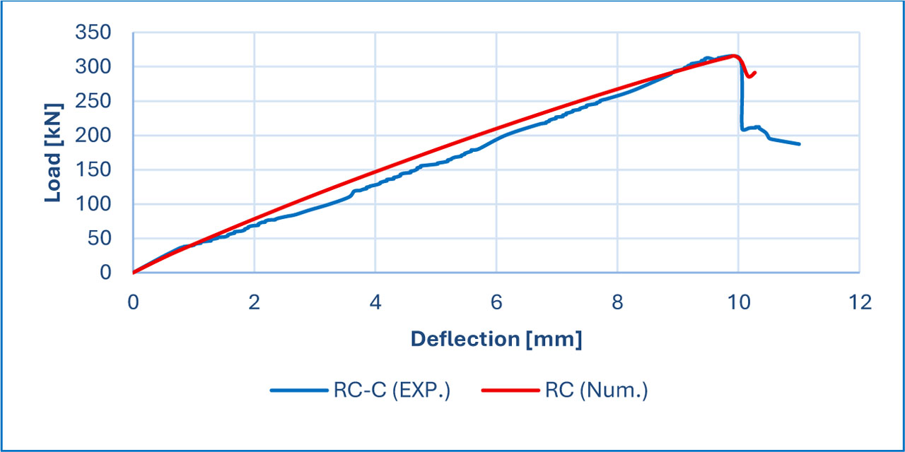
Figure 19:
Validation of (RC) sample
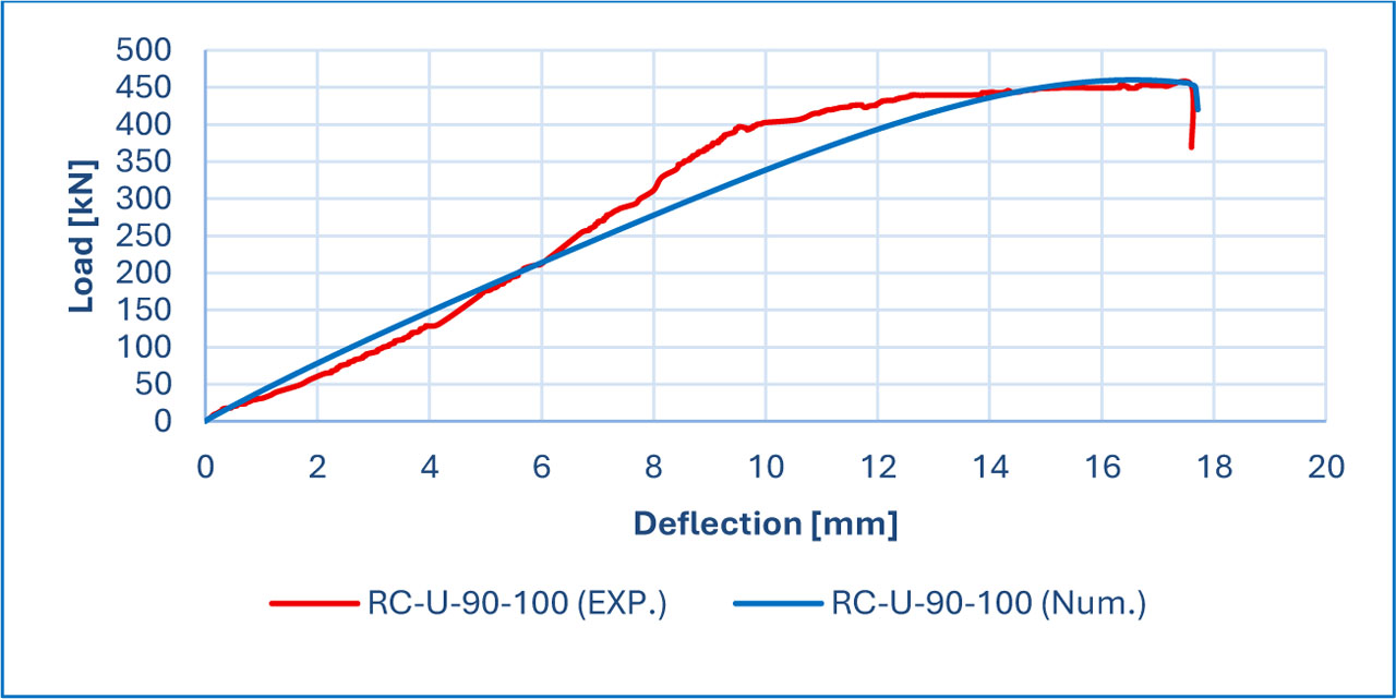
Figure 20:
Validation of (RC-CFRP-U-90-100) sample
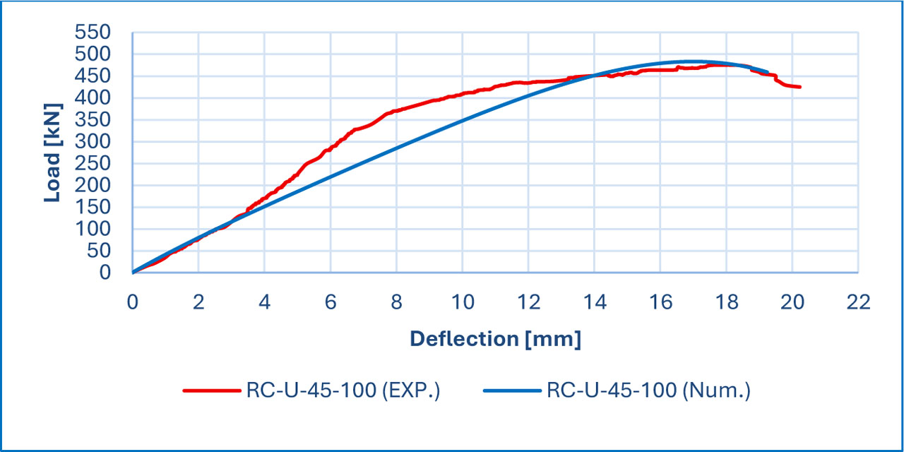
Figure 21:
Validation of (RC-CFRP-U-45-100) sample
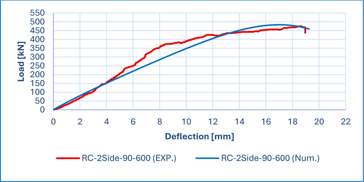
Figure 22:
Validation of (RC-CFRP-2SIDE-90-600) sample
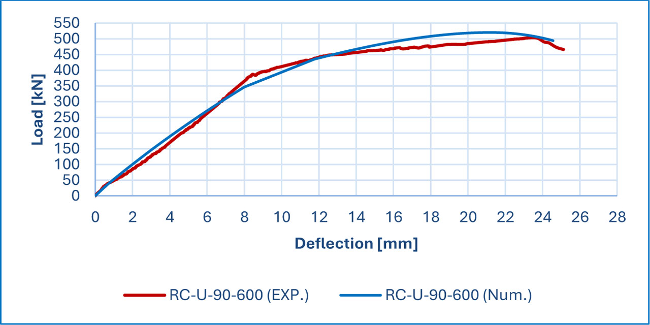
Figure 23:
Validation of (RC-CFRP-U-90-600) sample
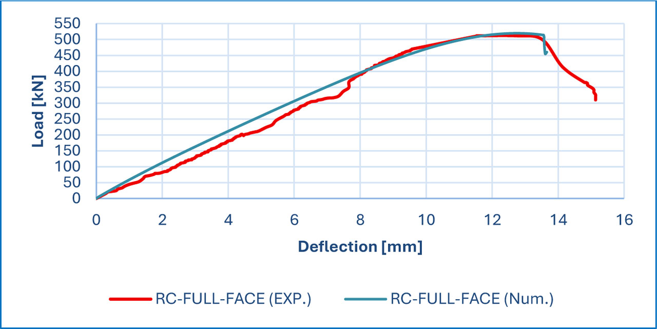
Figure 24:
Validation of (RC-CFRP-FULL-FACE) sample
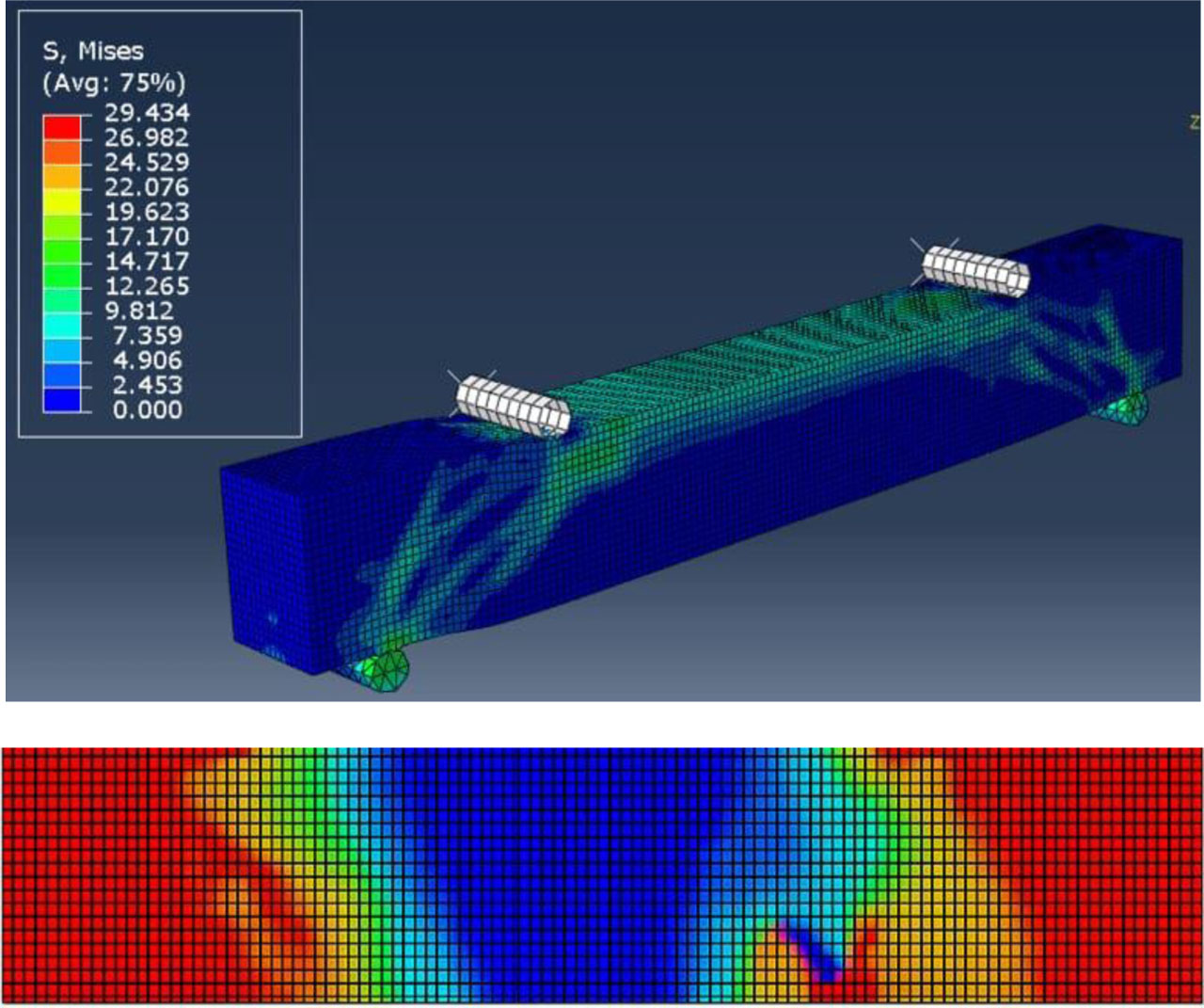
Figure 25:
Von Mises stress distribution and failure pattern of RC-CFRP-FULL-FACE beam model
7.2. Thickness
A new parameter, CFRP thickness, was introduced by evaluating two thicknesses: 0.167 mm (single layer) and 0.334 mm (double layer). The load–deflection behavior was captured and presented in Figures 26–30. The results in Table 9 indicate that increasing the CFRP thickness led to improved load capacity across all samples.
Table 9:
Summary for the thickness of the beam parameter
| Name of beam | Thickness 0.167mm | Thickness 0.334mm | Load increase [%] rate | ||
|---|---|---|---|---|---|
| Load [kN] | Deflection [mm] | Load [kN] | Deflection [mm] | ||
| RC-CFRP-U-90-100 | 459.90 | 16.54 | 512.24 | 18.34 | 11.38 |
| RC-CFRP-U-45-100 | 481.24 | 16.98 | 541.23 | 18.93 | 12.46 |
| RC-CFRP-2SIDE-90-600 | 483.24 | 16.92 | 543.65 | 18.85 | 12.50 |
| RC-CFRP-U-90-600 | 502.57 | 17.32 | 565.40 | 19.32 | 12.50 |
| RC-CFRP-FULL FACE | 519.46 | 12.73 | 621.75 | 15.27 | 19.69 |
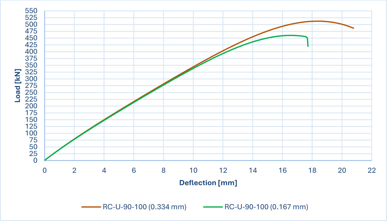
Figure 26:
Thickness of CFRP compares for the (RC-CFRP-U-90-100) sample
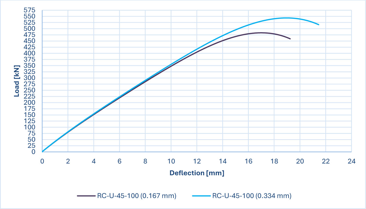
Figure 27:
The thickness of CFRP compared for the (CFRP-U-45-100) sample
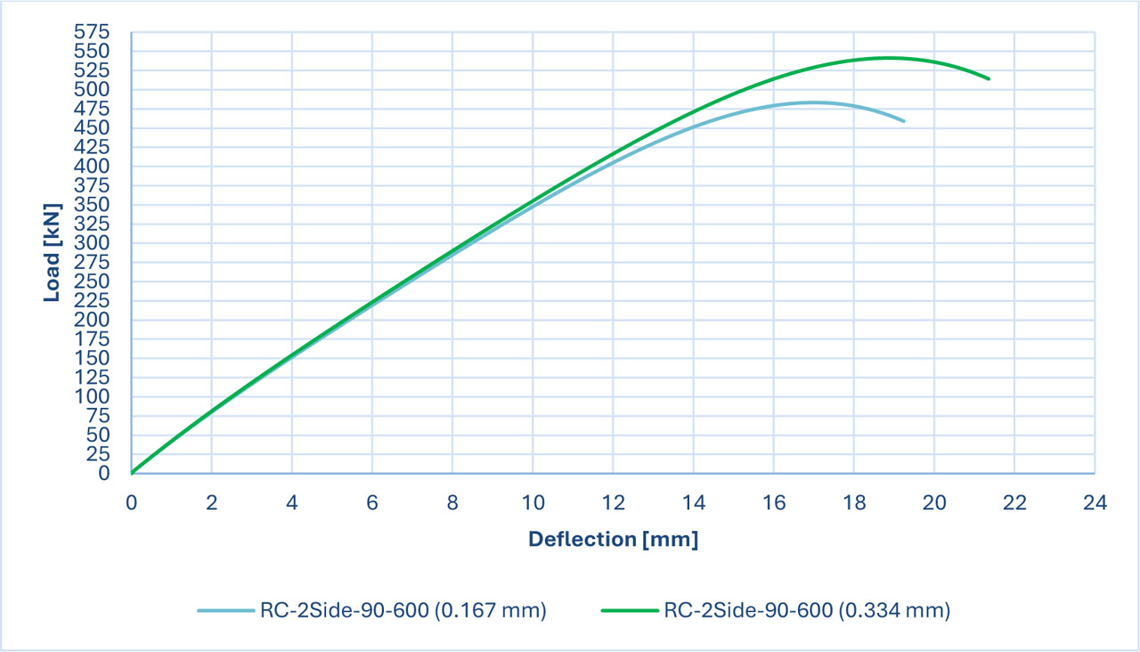
Figure 28:
The thickness of CFRP compared for the (RC-CFRP-2SIDE-90-600) sample
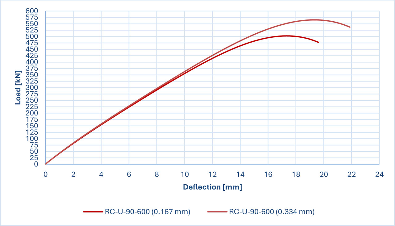
Figure 29:
The thickness of CFRP compared for the (CFRP-U-90-600) sample
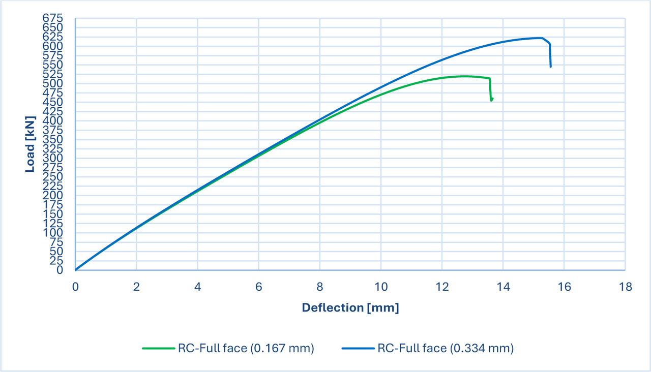
Figure 30:
The thickness of CFRP compared for the (RC-CFRP-FULL-FACE) sample
7.3. CFRP Spacing
The influence of CFRP strip spacing was examined by comparing samples RC-CFRP-U-90-100 and RC-CFRP-U-90-600, where both distance and strip width were varied. The load–deflection curves for these samples are illustrated in Figure 31.
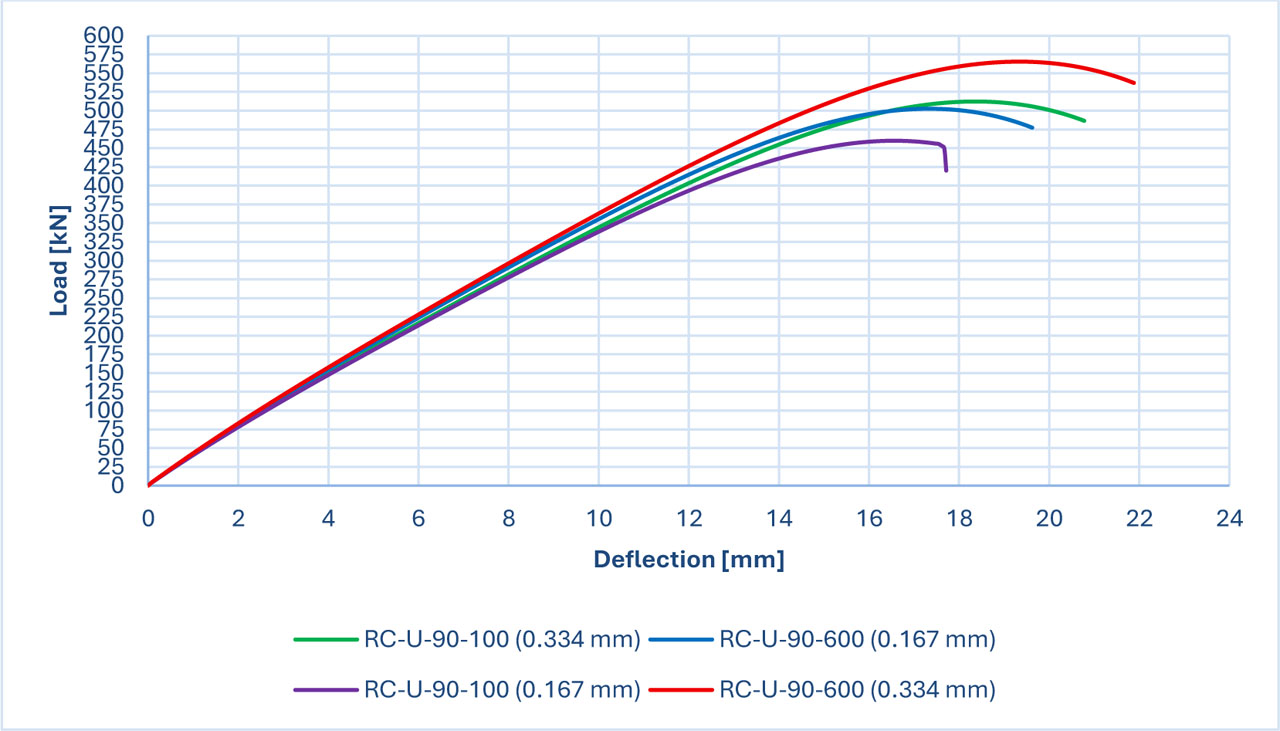
Figure 31:
Load deflection charts for the samples with CFRP spacing parameter
7.4. Combined Effect of Thickness and Spacing
Two different spacing values (150 mm and 200 mm) were combined with two CFRP thicknesses (0.167 mm and 0.334 mm) to study their joint effect on beam performance.
7.4.1. Spacing 200mm (thickness 0.167–0.334) mm
Table 10 and Figures 32, 33 show that increased thickness improves performance, with a higher gain observed at 45° fiber orientation than at 90°.
Table 10:
Summary for the thickness of the beam parameter
| Name of beam | Thickness 0.167mm | Thickness 0.334mm | Load increase rate [%] | ||
|---|---|---|---|---|---|
| Load [kN] | Deflection [mm] | Load [kN] | Deflection [mm] | ||
| RC-CFRP-U-90-100 | 298.94 | 10.17 | 352.74 | 12.51 | 18 |
| RC-CFRP-U-45-100 | 361.70 | 12.63 | 410.45 | 13.78 | 13.48 |
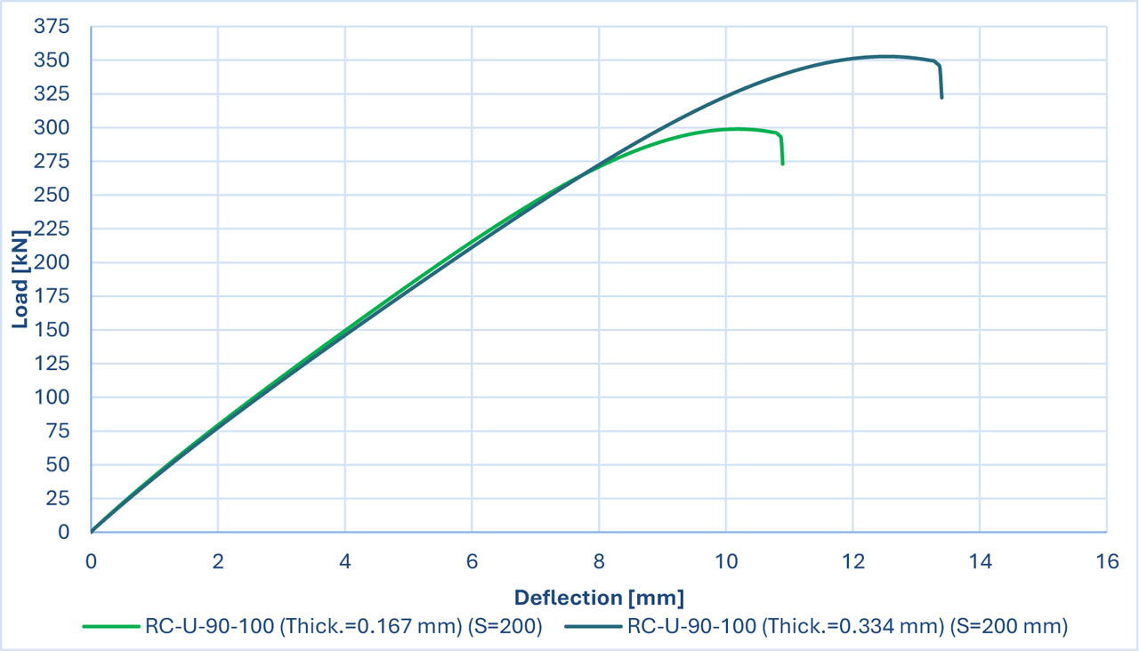
Figure 32:
Load deflection charts for the (RC-U-90-100) specimen with CFRP spacing (200 mm)
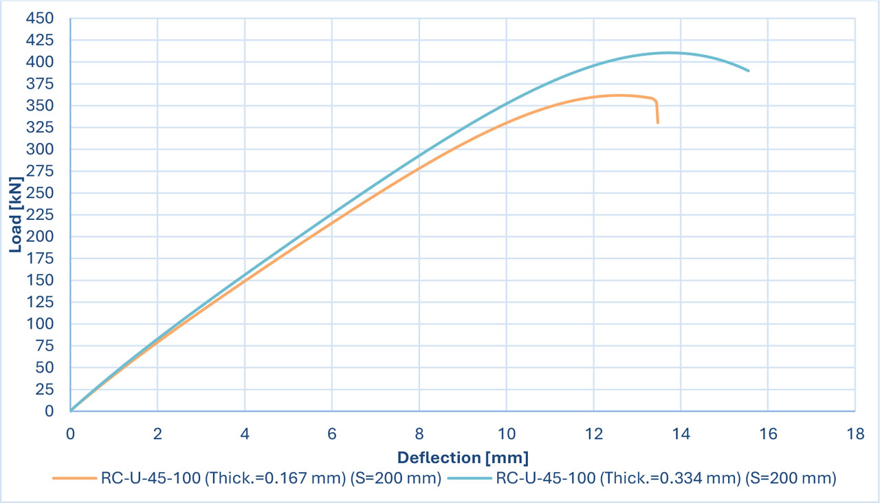
Figure 33:
Load deflection charts for the (RC-U-45-100) specimen with CFRP spacing (200 mm)
7.4.2. Spacing 150mm (thickness 0.167–0.334) mm
Table 11 and Figures 34, 35 show similar gains in both orientations, but the increase was more limited, indicating a reduced effect of added thickness at closer strip spacing.
Table 11:
Summary for the thickness of the beam parameter
| Name of beam | Thickness 0.167mm | Thickness 0.334mm | Load increase rate [%] | ||
|---|---|---|---|---|---|
| Load [kN] | Deflection [mm] | Load [kN] | Deflection [mm] | ||
| RC-CFRP-U-90-100 | 459.90 | 16.54 | 512.24 | 18.34 | 11.38 |
| RC-CFRP-U-45-100 | 483.24 | 17.05 | 543.65 | 19.01 | 12.46 |
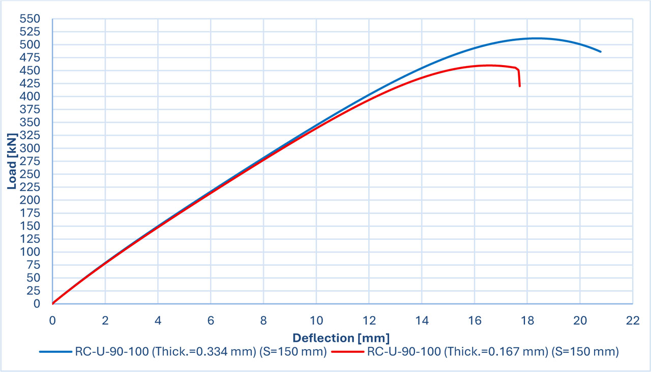
Figure 34:
Load deflection charts for the (RC-U-90-100) specimen with CFRP spacing (150 mm)
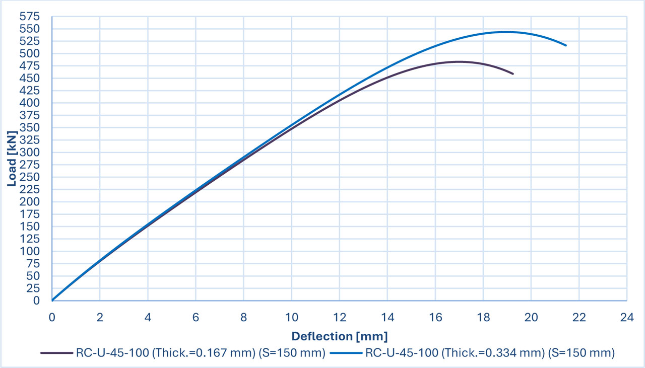
Figure 35:
Load deflection charts for the (RC-U-45-100) specimen with CFRP spacing (150 mm)
8. Discussion
8.1. General
The validation results confirm the accuracy of the finite element model in simulating the behavior of both control and CFRP-strengthened UHPC beams. The close match between the model and reference data in terms of load capacity and failure mode suggests that the numerical model reliably captures the key mechanical behavior.
Regarding the effect of thickness, all strengthened models exhibited improved performance with double-layer CFRP, although the percentage increase diminished with each additional layer. This indicates a point of diminishing returns where added material results in only minor strength gains. The fully wrapped model, however, stood out with the highest improvement (19.69%), confirming the efficiency of full-face strengthening in shear performance.
The spacing parameter also had a significant impact. Wider spacing (e.g., 600 mm) reduced the contribution of CFRP strips, while closer spacing (150 mm) provided better coverage but did not necessarily produce a proportional increase in strength. This suggests that optimal spacing should balance material use with structural efficiency.
When analyzing the combined effects of thickness and spacing, the results confirmed that slanted fiber orientation (45°) performed better than vertical (90°) in resisting shear forces. At 200 mm spacing, the influence of fiber angle was more prominent, while at 150 mm, the effect was less significant due to the higher confinement already provided by the closely spaced strips.
These findings indicate that CFRP configuration—particularly thickness, spacing, and fiber angle—must be carefully selected to achieve the most effective strengthening outcome in UHPC beams under shear loading.
8.2. Quantitative Discussion on Simulation Error and Model Limitations
To assess the accuracy of the finite element (FE) model, validation was performed by comparing the simulated load–deflection responses with those obtained experimentally for all beam configurations. As shown in Figures 19 to 24, the numerical results demonstrated a close agreement with the reference experimental data in terms of both ultimate load and deflection patterns. The average percentage difference in peak load between simulation and experiment across all samples was found to be within 5–8%, which is considered acceptable for nonlinear structural modeling involving composite materials.
Additionally, Figure 25 illustrates the von Mises stress distribution and predicted failure mode of the RC-CFRP-FULL-FACE beam, which closely matched the observed experimental failure mechanism, further confirming the model’s reliability. However, some limitations in the numerical approach must be acknowledged. First, the model assumes perfect bond between the CFRP sheets and the concrete substrate, whereas in reality, interface debonding and local slippage may occur and are difficult to capture without introducing a complex cohesive zone model. Second, the concrete was modeled using a homogeneous material model with isotropic damage properties, which does not fully reflect the localized cracking behavior, especially near load and support points. Third, while the mesh sensitivity was considered in preliminary analysis, using finer meshes in high-stress concentration areas could further improve the prediction accuracy, particularly near CFRP-concrete interaction zones.
Finally, boundary conditions and loading were applied in a quasi-static, load-controlled manner. Any imperfections or load eccentricities in the actual experimental setup were not replicated in the simulation, which may partially explain the minor discrepancies between numerical and experimental results.
Despite these limitations, the overall error margin remained relatively small, and the model was found to be effective for parametric studies, including the influence of CFRP thickness and spacing (Figures 26–35). The trends observed in the simulations—such as increased load capacity with thicker CFRP layers and tighter spacing—were consistent with experimental observations and engineering expectations.
8.3. Review in the Context of Design Standards and Guidelines with experimental results
Existing structural design standards and guidelines, such as ACI 318-19, ACI 440.2R-17, TR-55, and CNR-DT-215-2018, serve as the primary references for structural engineering practices and provide methodologies for predicting the shear capacity of reinforced concrete beams, especially those strengthened with CFRP reinforcement. The outcomes of ACI 440.2R-17, TR-55, and CNR-DT-215-2018 enable the independent evaluation of CFRP’s contribution to shear resistance, distinguishing it from that of the concrete matrix. To assess the reliability of these design codes in predicting CFRP reinforcement effects in UHPC beams, the experimental results obtained through the subtraction analysis method (presented in Table 9) were compared with numerical predictions derived from the existing design standards. The consolidated findings are reported in Table 12. The comparison indicates that TR-55, and CNR-DT-215-2018 tend to accuracy the shear contribution of CFRP in U-shaped full-face reinforcement configurations while ACI 440.2R-17 tends to overestimate the shear contribution of CFRP in U-shaped full-face reinforcement configurations. This overestimation primarily arises from the way these codes incorporate concrete compressive strength into their predictive models for CFRP effectiveness. Yet, this approach fails to fully describe the relationship between CFRP and concrete in UHPC beams, since the efficiency of CFRP is affected by the bond length and how strong the concrete substrate is. When results from experiments are contrasted with existing design codes, it becomes obvious that better models are needed to predict the shear strength of carbon fibre-reinforced cement beams. Experiments show that the ACI 318-19 code gives the most correct results. The findings point out that considering effective CFRP bond length and variations in concrete’s tensile strength greatly improves the accuracy of design calculations. Future studies should upgrade shear prediction models to pay attention to such important factors, resulting in safer and more economical layouts for CFRP-strengthened UHPC structures.
Table 12:
Observed versus estimated shear contributions of CFRP in the strengthened specimens
| Specimens | CFRP Contribution Determined by the Subtraction approach: [kN] | CFRP Contribution According to ACI 440.2R-17: [kN] | CFRP Contribution According to CNR-DT-215-2018: [kN] | CFRP Contribution According to TR-55 (CS, 2013): [kN] |
|---|---|---|---|---|
| RC-U-90-100 | 70.110 | 73.132 | 57.234 | 63.593 |
| RC-U-45-100 | 80.615 | 103.698 | 57.234 | 89.934 |
| RC-2side-90-600 | 80.900 | 109.698 | 85.851 | 95.390 |
| RC-U-90-600 | 95.090 | 109.698 | 85.851 | 95.390 |
| RC-Full-Face | 99.120 | 109.698 | 85.851 | 95.390 |
9. Conclusion
Inclusion This paper included a detailed study of how UHPC beams reinforced by CFRP behave under shear, considering different ways in which the materials are arranged and located in the beams. Through experimental and numerical studies, we discovered important results about the effectiveness of CFRP reinforcement that can now inform structural design codes. Whenever closed-shaped CFRPs were used in beams, they showed a much higher strain capacity than U-shaped configurations, where CFRP came loose at the interface and reduced the beam’s shear capacity greatly. In comparison, the closed configuration of CFRP resulted in much better closure and high shear resistance.
Predictions relying on codes tended to overstate the shear contribution of CFRP, mainly when the section formed a U-shaped bracket. The main reason for the discrepancy is the short bond length between CFRP and UHPC surface, affected by the concrete tensile strength, which is not considered enough by the current models, leading to less accurate shear predictions for UHPC beams. The results prove that making changes to current design standards is necessary to support CFRP-strengthened UHPC beams in practice. Most of the present codes were developed using typical concrete data, making them suitable for few UHPC usage cases.
Additional analysis and research on the bond mechanisms within FRP and UHP concrete are needed to increase how reliable and efficient such reinforcement is. This research highlights the role of correctly characterizing CFRP when used in U-shaped reinforcement, as debonding can make performance unstable. Adjusting design techniques to look at bond length, tension in concrete and CFRP bolts will result in better predictions for shear capacities and failure types in UHPC concrete supported by CFRP. Stronger and more reliable use of CFRP in concrete building will be made safer with increased research.
In this thesis, new FEA and analytical models were established to examine the response of the FRP/uhpc concrete connections. The results of FEA and the analytical proposed models show how these models can be used to predict the behaviour of the FRP/concrete joint reasonable accuracy. Based on tests carried on the experimental model, the finite element tests and analytical several conclusions can be drawn based on the models
Predictions of the shear response and failure patterns of were performed by means of 3D finite element models. the uhpc beams enhanced in shear reinforced with CFRP strips. The common reaction of the FE models depicts reasonable correspondence of the predictions with the test results (experimental). Overall, the finite element models are stiffer responding than the experimentally loaded ones. samples. This was attributed to the loss of the bond between the longitudinal steel reinforcement. This is due to the concrete in the actual case that is not modelled in the finite element models that are simulated in this. study. In addition, the inability to mathematically model concrete discrete cracks in a simulated fashion makes the FEA models stiffer than the real physical models. Shear failure mechanisms of the RC beams are highly complicated particularly in retrofitted samples FRP reinforced concrete with. Summing up, it could be stated that the developed in the current research 3D cracking FE models can serve as an extra tool to examine the shear mechanism and how different factors affect the shear behaviour of LWRC beams that are retrofitted with CFRP reinforcement. As one can conclude, the FE modelling of the RSS system with the assistance of the TS50 amplifier was carried out with satisfactory accuracy. The philosophy will come in handy with CFRP reinforcing in general.
Acknowledgements
I would like to extend my sincere thanks to Dr. Mustafa Hamid Farhan, for his exceptional efforts in contributing to the analysis of the results. I also thank the Civil Engineering Department laboratories at the university for the facilities and flexibility they provided in using the equipment. I also thank everyone who contributed to the success of this work.