
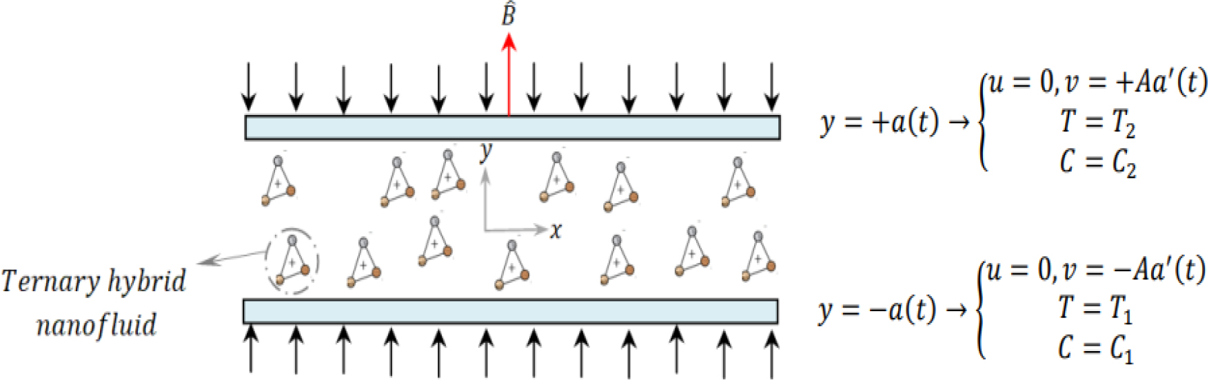
Fig. 1.
Physical model
Tab. 1.
A characteristic made between the physical features of ternary hybrid nanofluids.
| Dynamic viscosity | |
| Density | |
| Specific heat | |
| Electrical Conductivity | |
| Thermal Conductivity |
Tab. 2.
Thermophysical characteristics of a ternary hybrid nanofluid
| Physical properties | ρ (kg/m3) | Cp(J/kg. °K) | k(W/m.°K) | σ(S/m) |
|---|---|---|---|---|
| Blood | 1063.8 | 3594 | 0.492 | 0.8 |
| TiO2 → φ1 | 4250 | 397.2 | 8.9538 | 2.4×10+6 |
| SiO2 → φ2 | 2200 | 765 | 1.4013 | 3.5×10+6 |
| Al2O3 → φ3 | 3970 | 686 | 40 | 36.9×10+6 |
Tab. 3.
Explanation of the parameter control constraints
| Symbol | Name | Formula |
|---|---|---|
| α | Time-dependent dimensionless parameter | |
| Re | Reynolds number | |
| Sc | Schmidt numbers | |
| Ec | Eckert number | |
| M | Hartmann number | |
| Pr | Prandtl number | |
| Br | Brinkman number | Pr ∗ Ec |
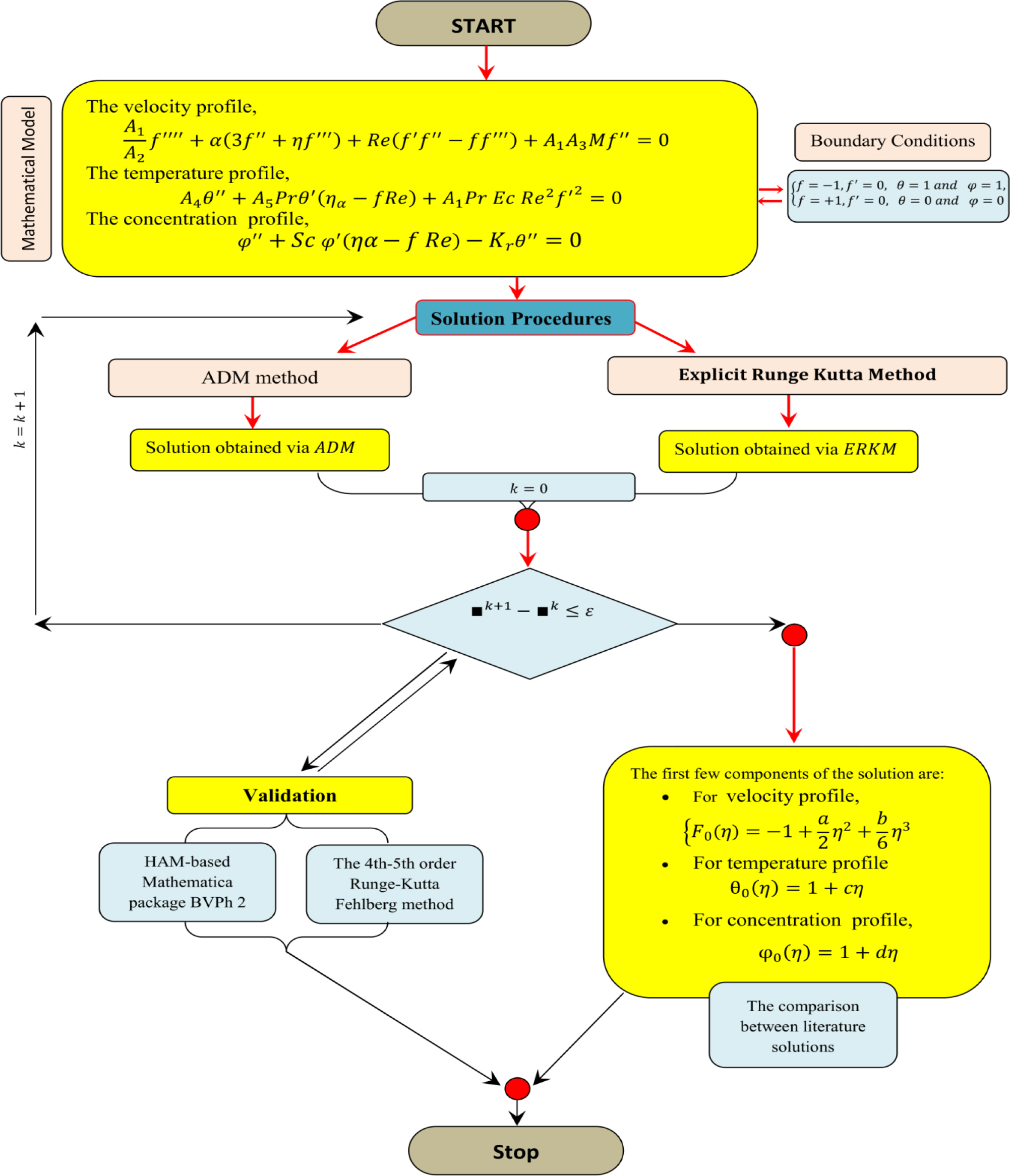
Fig. 2.
ADM procedure
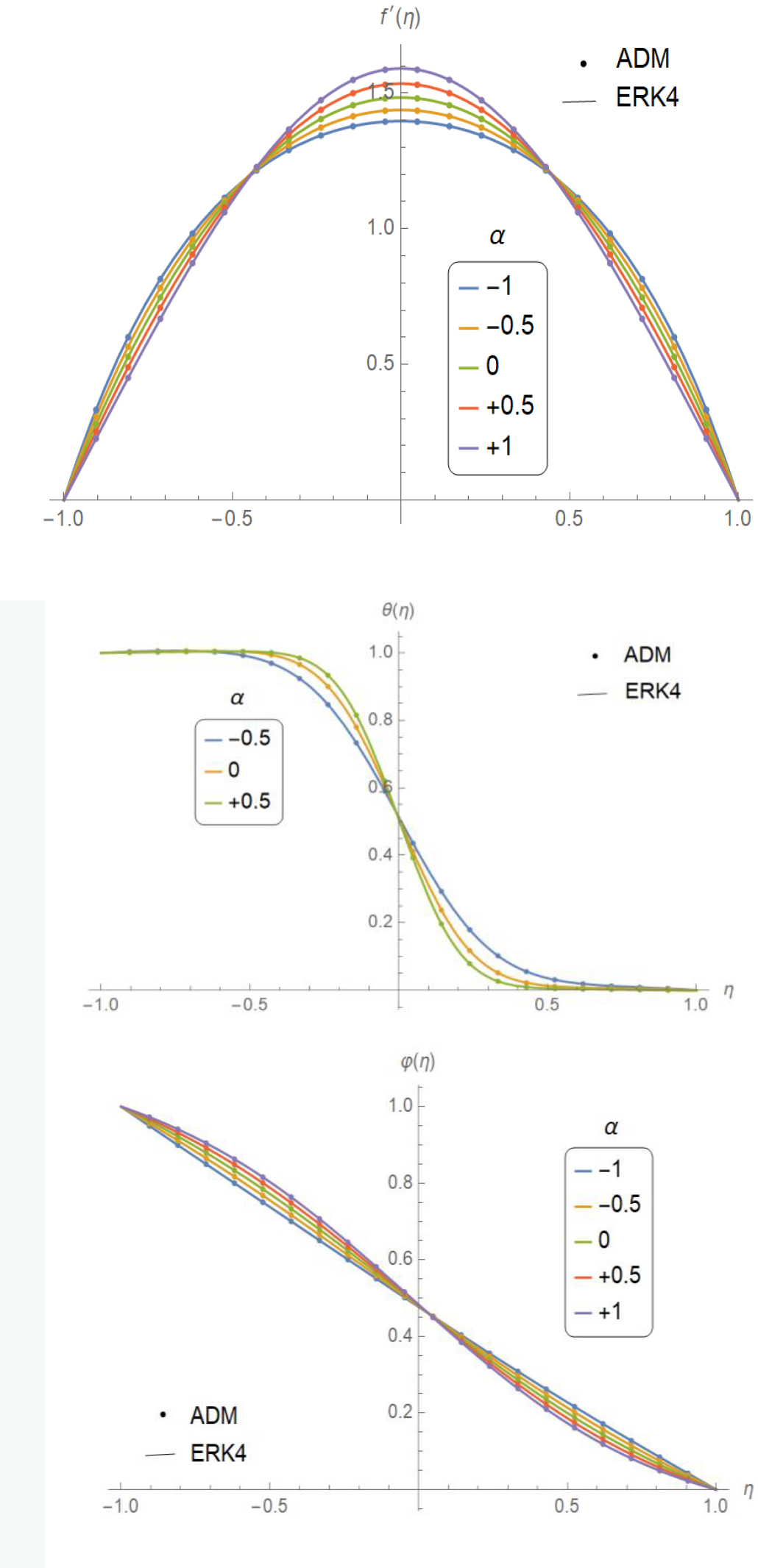
Fig. 3.
Influence of α on f′, θ and φ when: φ1 = φ2 = φ3 = 0.01, Re = –1, M = 1, Sc = 1, Kr = 0.1 and Pr = 21
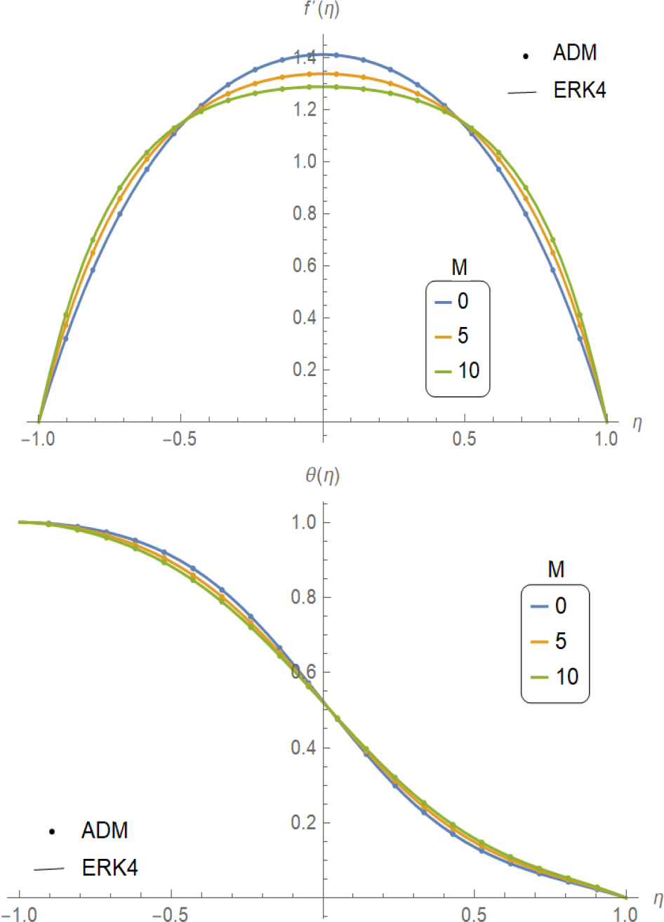
Fig. 4.
Influence of M on f′ and θ when: φ1 = φ2 = φ3 = 0.01, Re = –1, α = –1, Sc = 1, Kr = 0.1 and Pr = 21
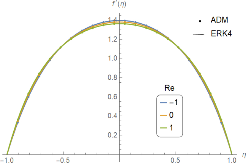
Fig. 5.
Influence of fie on f′ when: φ1 = φ2 = φ3 = 0.01, α = –1, Sc = 1, Kr = 0.1 and Pr = 21
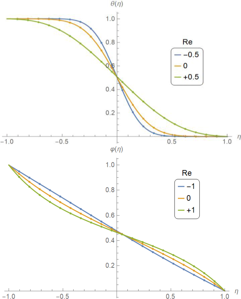
Fig. 6.
Influence of fie on θ(η) and φ(η) when: φ1 = φ2 = φ3 = 0.01, φ = –1, Sc = 1, Kr = 0.1 and Pr = 21
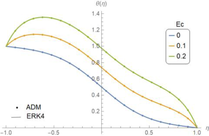
Fig. 7.
Influence of Ec on θ when: φ1 = φ2 = φ3 = 3 = 0.01, Re = –1, α = –1, Sc = 1 and Kr = 0.1
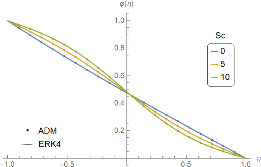
Fig. 8.
Influence of Sc on θ when: φ1 = φ2 = φ3 = 0.01, Re = –1, α = – 1, M = 1, Kr = 0.1 and Pr = 21
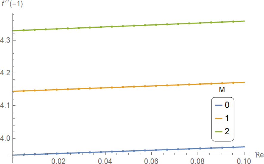
Fig. 9.
Influence of both Re and M on f″ when: φ1 = φ2 = φ3 = 0.01, Re = –1, α = –1, Kr = 0.1 and Pr = 21
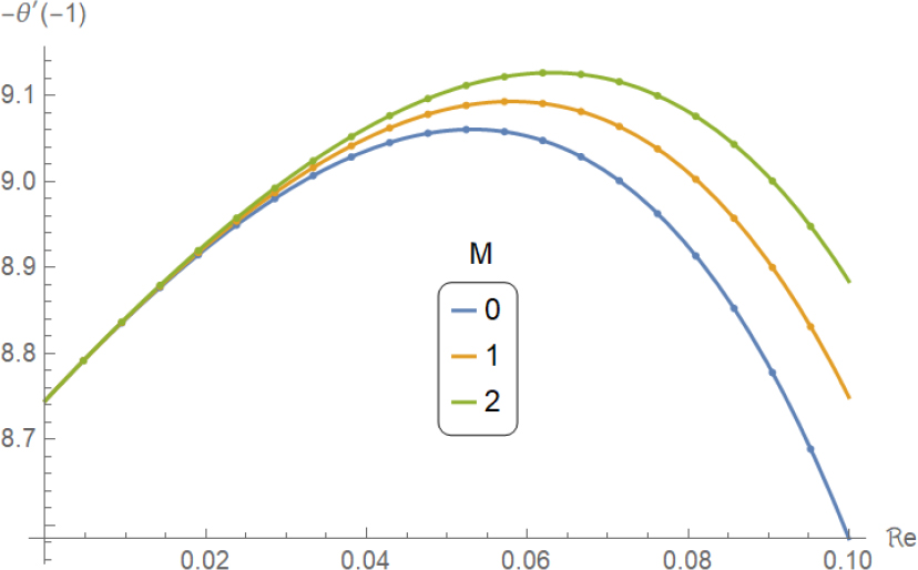
Fig. 10.
Influence of both Re and M on θ′(–1) when: φ1 = φ2 = φ3 = 0.01, α = –1, Kr = 0.1 and Pr =21
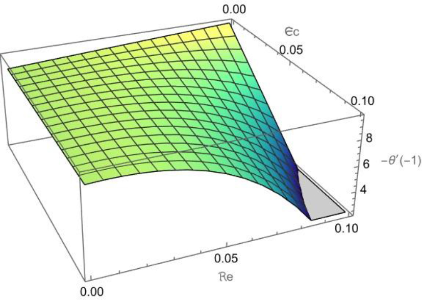
Fig. 11.
Influence of both Re and Ec on –θ′(–1) when: φ1 = φ2 = φ3 = 0.01, α = –1, Kr = 0.1 M = 1 and Pr = 21
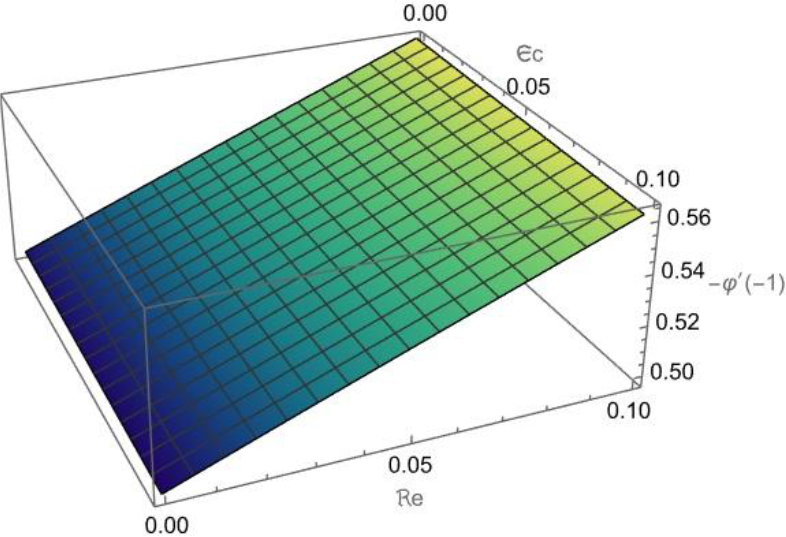
Fig. 12.
Influence of both Re and Ec on φ′(–1) when: φ1 = φ2 = φ3 = 0.01, α = –1, Kr = 0.1 M = 1 and Pr = 21
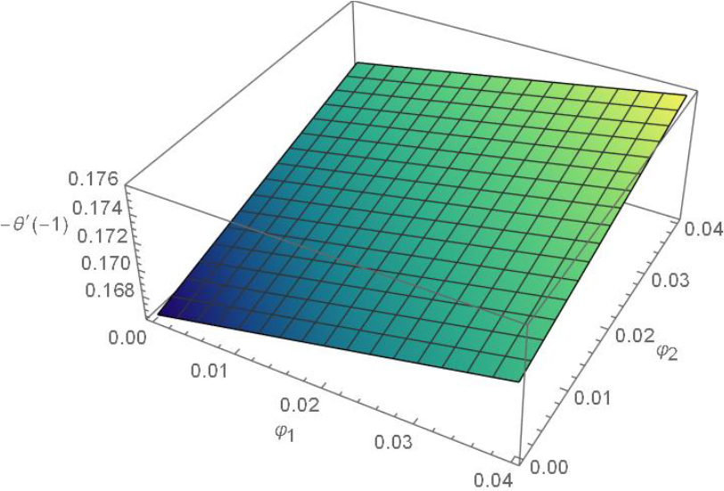
Fig. 13.
Influence of both φ1 and φ2 on φ′(–1) when: Re = –1, Ec = 0.01, φ3 = 0.01, α = –1, Kr = 0.1 M = 1 and Pr = 21
Tab. 5.
Effects of φ on the f′(0) and θ(0) when Re = α = –1, Kr = M = Sc = 1 and Pr = 21
| φTiO2 | φSiO2 | φAl2O3 | f″(–1) | θ′(–1) | |
|---|---|---|---|---|---|
| N-F | 0% | 0% | 0% | 1.4067241 | 0.5258221 |
| 2% | 0% | 0% | 1.3993983 | 0.52438206 | |
| 0% | 2% | 0% | 1.4016671 | 0.5247220 | |
| 0% | 0% | 2% | 1.3987235 | 0.52430242 | |
| φTiO2 | φSiO2 | φAl2O3 | f″(–1) | θ′(–1) | |
| HN-F | 0% | 0% | 0% | 1.4067241 | 0.5258221 |
| 2% | 2% | 0% | 1.3941953 | 0.52334135 | |
| 0% | 2% | 2% | 1.39345981 | 0.5232619 | |
| 2% | 0% | 2% | 1.39123039 | 0.522949 | |
| φTiO2 | φSiO2 | φAl2O3 | f″(–1) | θ′(–1) | |
| THN-F | 0% | 0% | 0% | 1.4067241 | 0.5258221 |
| 1% | 1% | 1% | 1.3965176 | 0.52382605 | |
| 2% | 2% | 2% | 1.3858312 | 0.52196548 | |
| 0% | 0% | 2% | 1.3746924 | 0.52023433 |
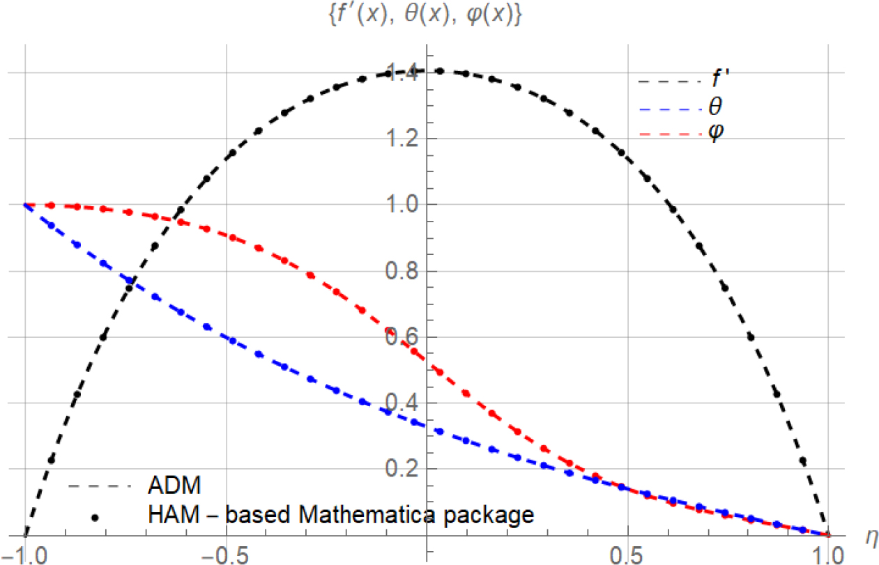
Fig. 14.
Comparison of f′, θ and φ with HAM-package when : Re = α = –1, Kr = M = Sc = 1 and Pr = 21
Tab. 6.
Comparison for f″(–1), θ′(–1) and φθ′(–1) when α = 1, φ = 0.06, Kr = 0.1, Ec = 0, M = 1, Sc = 1 and Pr = 6.2
| Symbol | Description | Units (if applicable) |
| A | Permeability constant | --- |
| Br | Brinkman number | --- |
| C | Concentration | mol/m3 |
| Cp | Specific heat capacity | J/kg·K |
| D | Mass diffusivity | m2/s |
| Ec | Eckert number | --- |
| f | Dimensionless velocity function | --- |
| M | Hartmann number | --- |
| Pr | Prandtl number | --- |
| Re | Reynolds number | --- |
| Sc | Schmidt number | --- |
| T | Temperature | K |
| u,v | Velocity components | m/s |
| α | Unsteadiness parameter | --- |
| η | Similarity variable | --- |
| θ | Dimensionless temperature | --- |
| μ | Dynamic viscosity | Pa·s |
| ρ | Density | kg/m3 |
| σ | Electrical conductivity | S/m |
| φ | Dimensionless concentration | --- |