
Tab. 1.
The chosen value of P, Q and R
| P | Q | R | F | |
|---|---|---|---|---|
| 1 | m2 | −(1 + m2) | 1 | sn, cd |
| 2 | −m2 | 2m2 − 1 | 1 − m2 | cn |
| 3 | −1 | 2 − m2 | m2 − 1 | dn |
| 4 | 1 | −(1 + m2) | m2 | ns, dc |
| 5 | 1 − m2 | 2m2 − 1 | −m2 | nc |
| 6 | m2 − 1 | 2 − m2 | −1 | nd |
| 7 | 1 − m2 | 2 − m2 | 1 | sc |
| 8 | −m2(1 − m2) | 2m2 − 1 | 1 | sd |
| 9 | 1 | 2 − m2 | 1 − m2 | cs |
| 10 | 1 | 2m2 − 1 | -m2(1 − m2) | ds |
| 11 | mcn ∓ dn | |||
| 12 | ns ∓ cs | |||
| 13 | nc ∓ sc | |||
| 14 | ns ∓ ns | |||
| 15 | ||||
| 16 | ||||
| 17 | ||||
| 18 | ||||
| 19 | ||||
| 20 | ||||
| 21 |
Tab. 2.
Analysis of Jacobi elliptic functions in the limit of m → 0 and m → 1.
| m → 1 | m → 0 | m → 1 | m → 0 | ||||
|---|---|---|---|---|---|---|---|
| 1 | snu | tanhu | sinu | 7 | dcu | 1 | secu |
| 2 | cnu | sechu | cosu | 8 | ncu | coshu | secu |
| 3 | dnu | sechu | 1 | 9 | scu | sinhu | tanu |
| 4 | cdu | 1 | cosu | 10 | nsu | cothu | cscu |
| 5 | sdu | sinhu | sinu | 11 | dsu | cschu | cscu |
| 6 | ndu | coshu | 1 | 12 | csu | cschu | cotu |
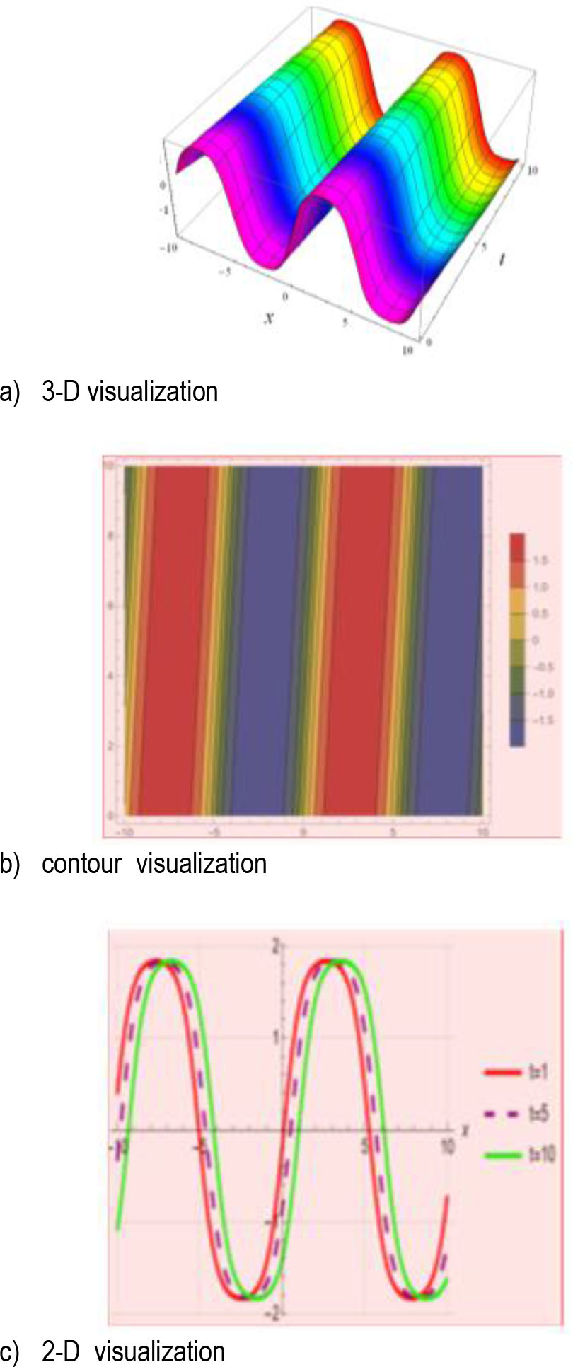
Fig. 1.
3-D, contour visualization and 2-D propagation of q1,1 for specific values of the parameters are ɛ = 1.2, α = 1.3, δ = 0.5, m = 0.9, c = 0.1
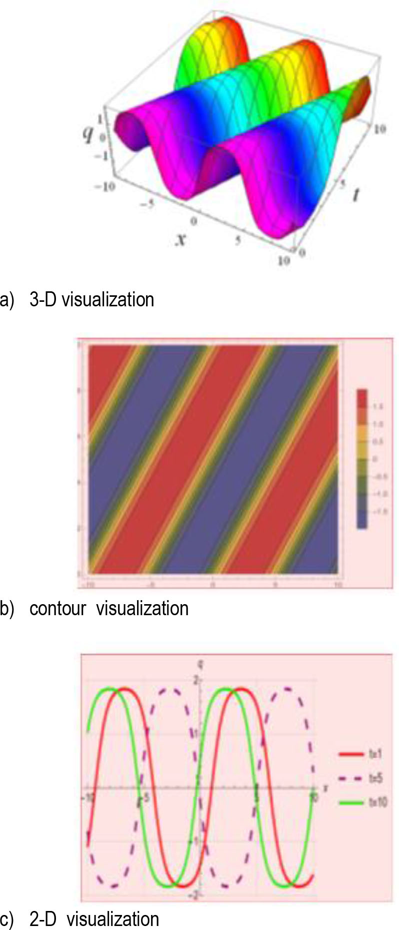
Fig. 2.
3-D, contour visualization and 2-D propagation of q1,1 for specific values of the parameters are ɛ = 1.2, α = 1.3, δ = 0.5, m = 0.9, c = 01
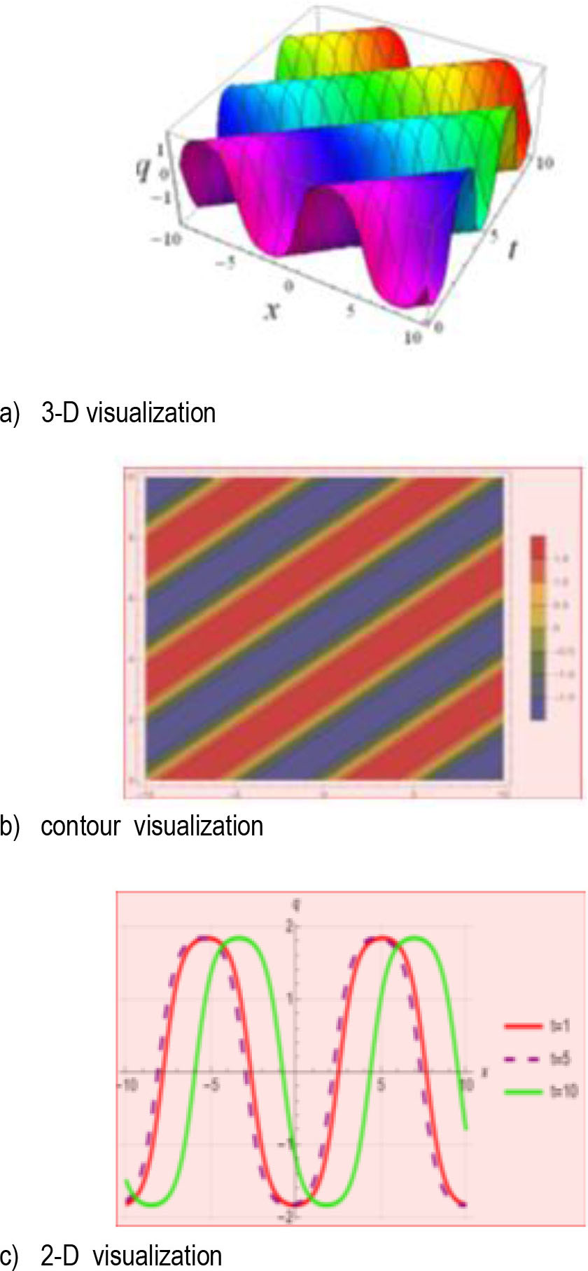
Fig. 3.
3-D, contour visualization and 2-D propagation of q1,1 for specific values of the parameters are ɛ = 1.2, α = 1.3, δ = 0.5, m = 0.9, c = 2.5
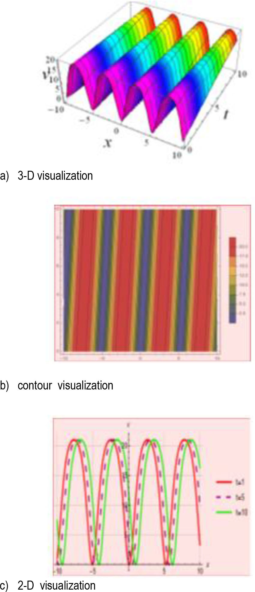
Fig. 4.
3-D, contour visualization and 2-D propagation of ν1,1 for specific values of the parameters are ɛ = 1.2, α = 1.3, δ = 0.5, n = 1.5, c = −1.5, m = 0.9, c = 0.1.
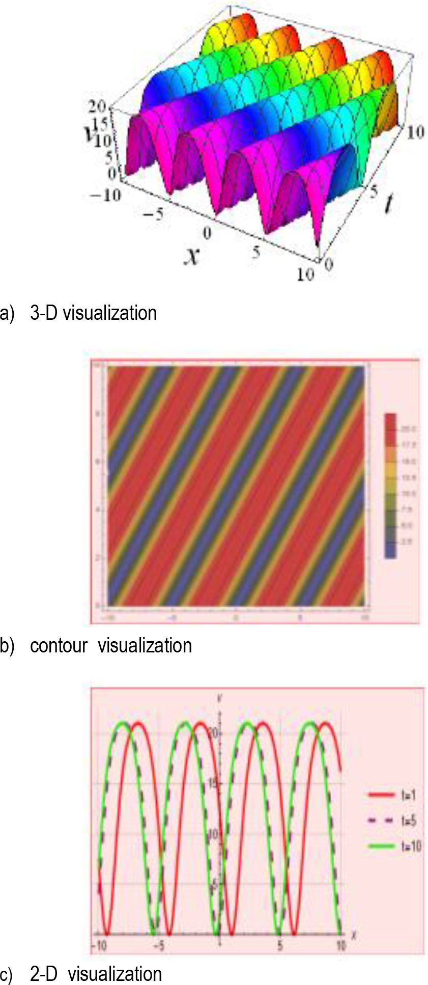
Fig. 5.
3-D, contour visualization and 2-D propagation of ν1,1 for specific values of the parameters are ɛ = 1.2, α = 1.3, δ = 0.5, n = 1.5, c = −1.5, m = 0.9, c = 01
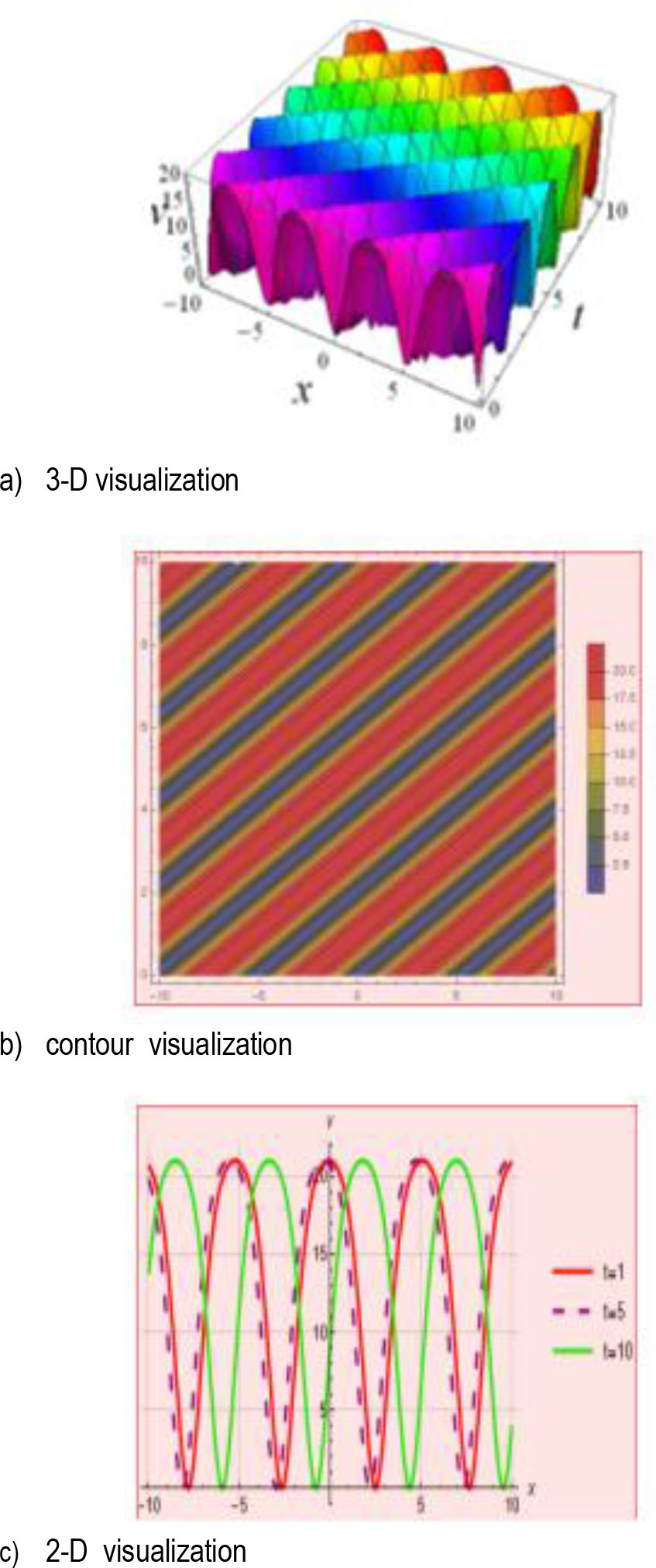
Fig. 6.
3-D, contour visualization and 2-D propagation of ν1,1 for specific values of the parameters are ɛ = 1.2, α = 1.3, δ = 0.5, n = 1.5, c = −1.5, m = 0.9, c = 2.5
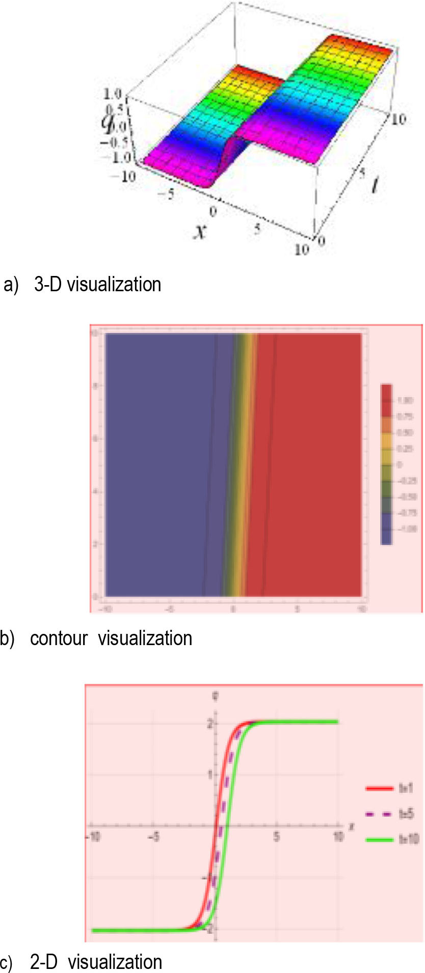
Fig. 7.
3-D, contour visualization and 2-D propagation of q1,2 for specific values of the parameters are ɛ = 1.2, α = 1.3, δ = 0.5, m = 0.5, c = 0.1
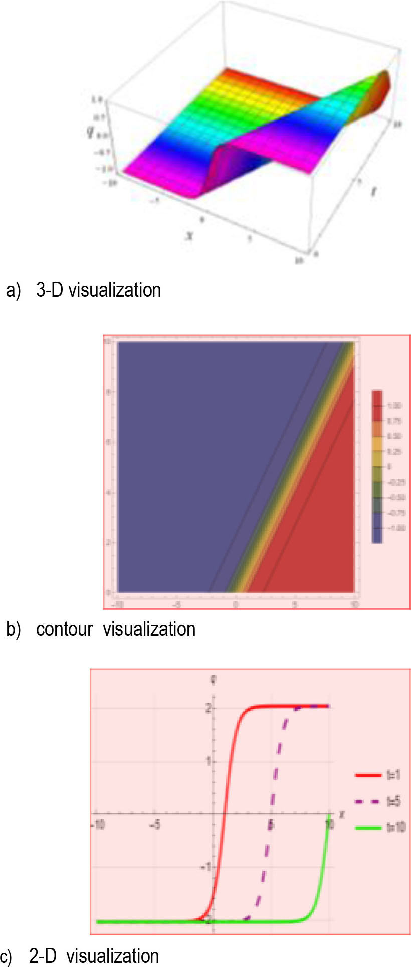
Fig. 8.
3-D, contour visualization and 2-D propagation of q1,2 for specific values of the parameters are ɛ = 1.2, α = 1.3, δ = 0.5, m = 0.5, c = 01
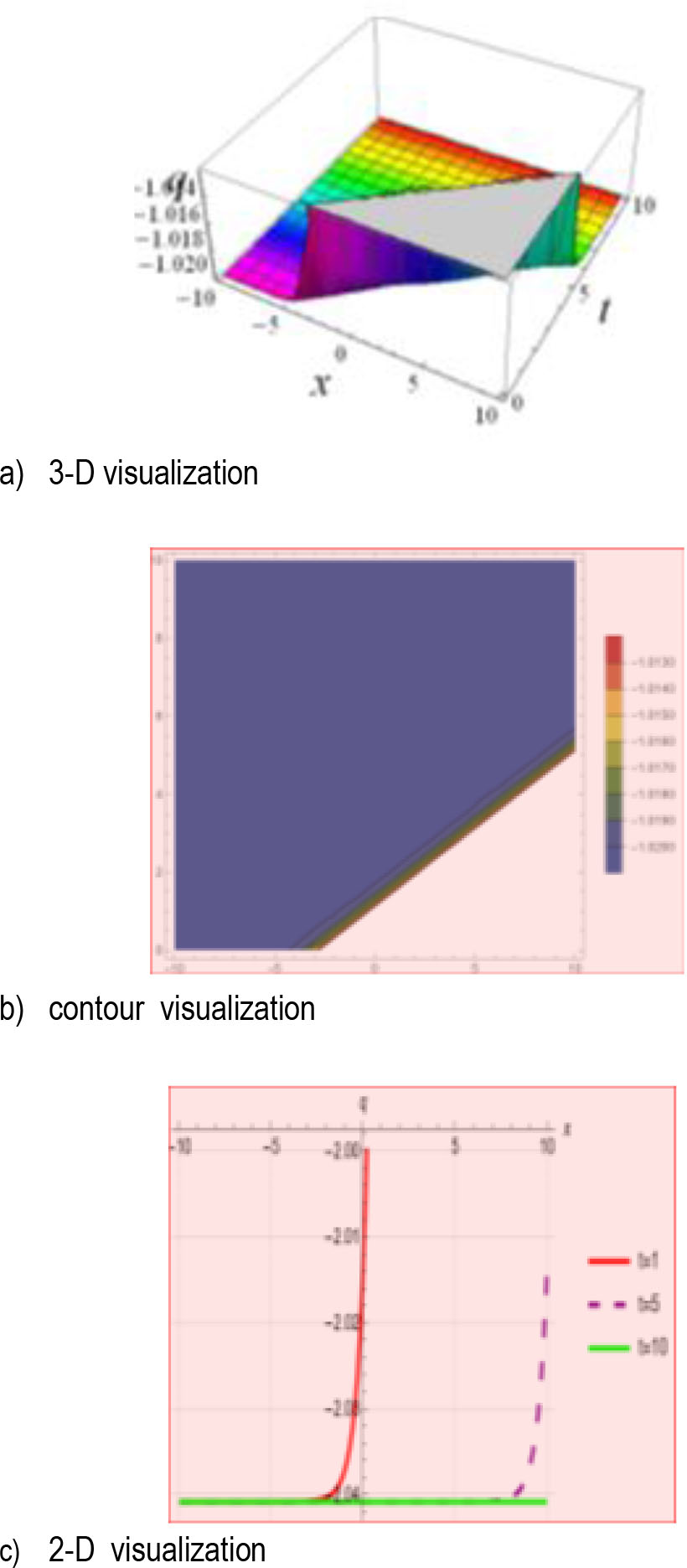
Fig. 9.
3-D, contour visualization and 2-D propagation of q1,2 for specific values of the parameters are ɛ = 1.2, α = 1.3, δ = 0.5, m = 0.5, c = 2.5
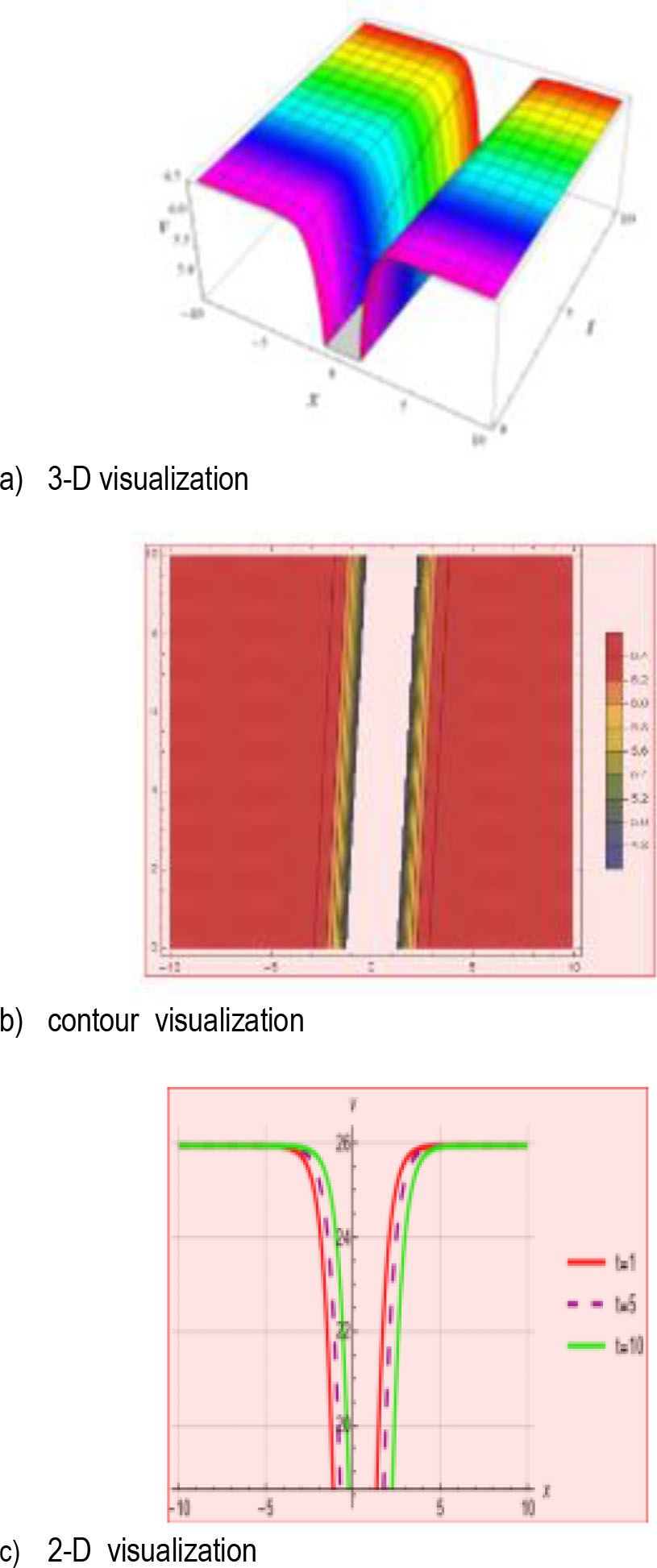
Fig. 10.
3-D, contour visualization and 2-D propagation of ν1,2 for specific values of the parameters are ɛ = 1.2, α = 1.3, δ = 0.5, n = 1.5, c = −1.5, m = 0.5, c = 0.1
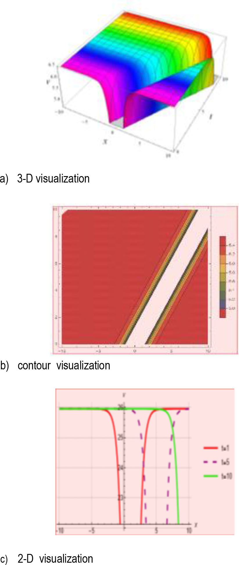
Fig. 11.
3-D, contour visualization and 2-D propagation of ν1,2 for specific values of the parameters are ɛ = 1.2, α = 1.3, δ = 0.5, n = 1.5, c = −1.5, m = 0.5, c = 01
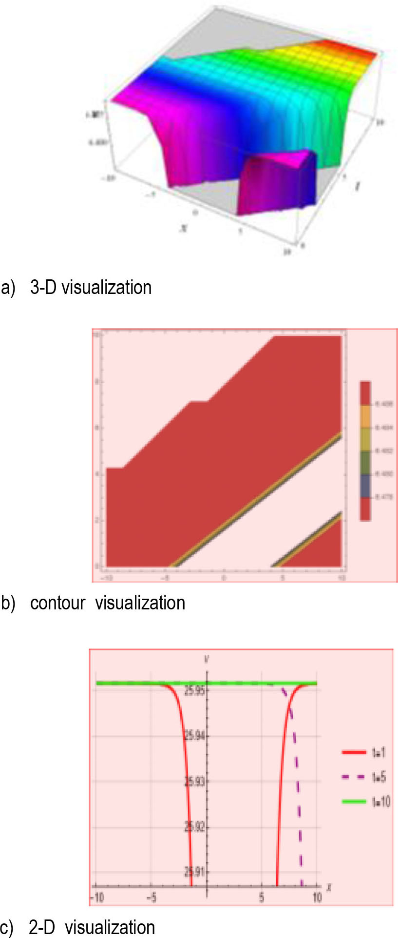
Fig. 12.
3-D, contour visualization and 2-D propagation of ν1,2 for specific values of the parameters are ɛ = 1.2, α = 1.3, δ = 0.5, n = 1.5, c = −1.5, m = 0.5, c = 2.5