
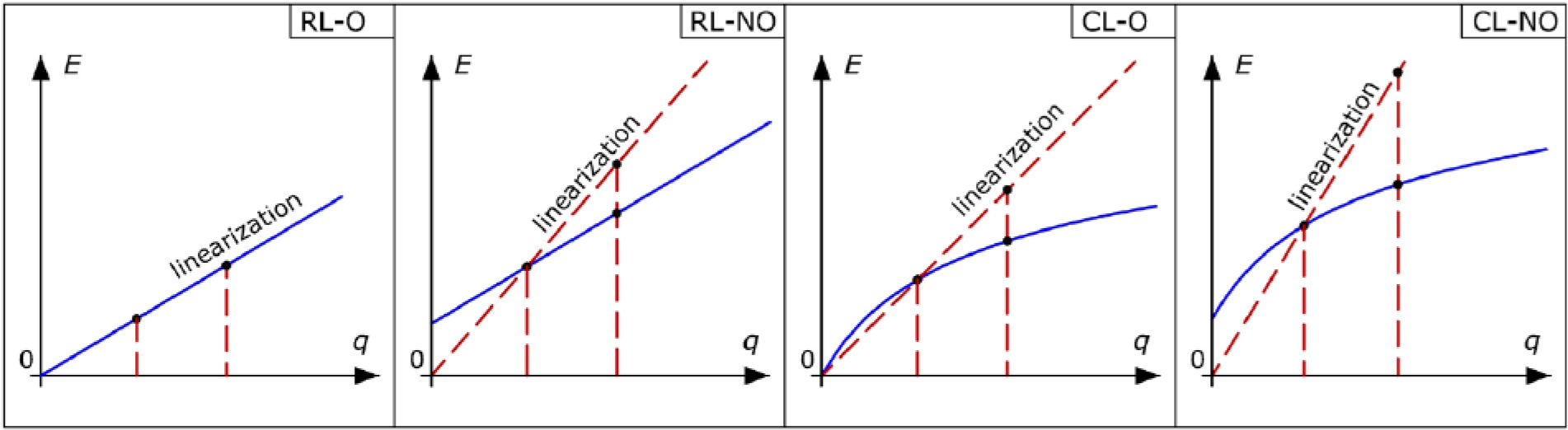
Figure 1.
Various forms of linear/nonlinear relations E(q)
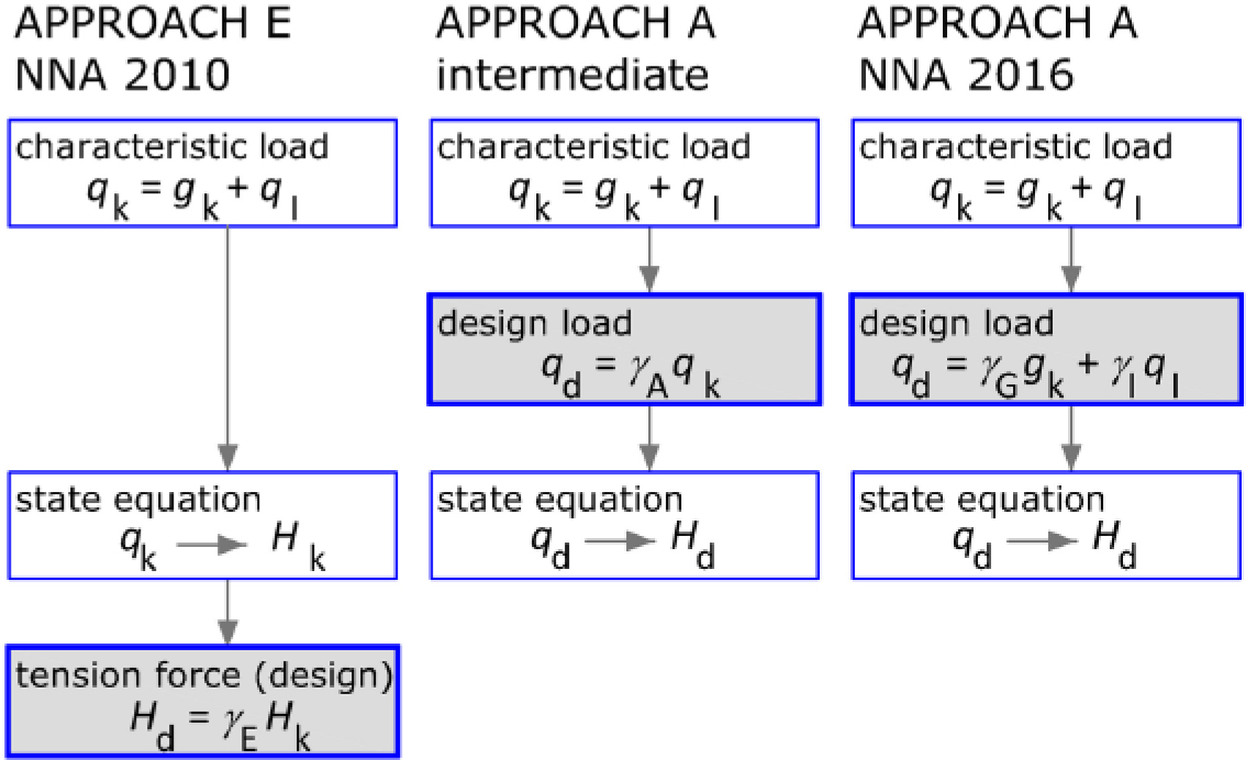
Figure 2.
Diagram illustrating approaches related to PSF application for design tension forces
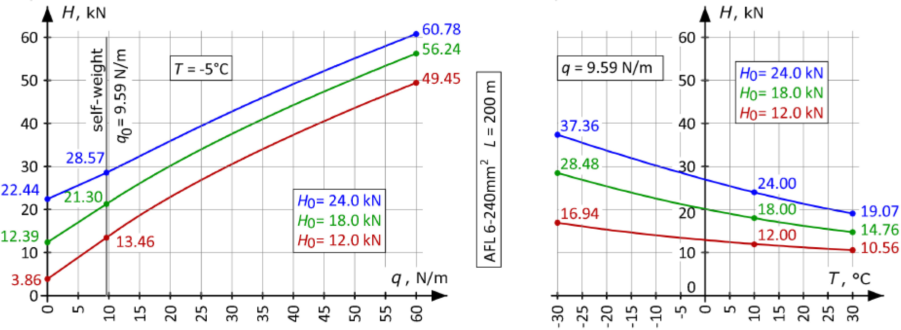
Figure 3.
Relationships H(q) and H(T) for conductor AFL-6 240 mm2
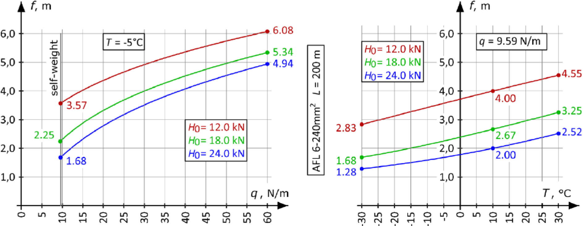
Figure 4.
Relationships f(q) and f(T) for conductor AFL-6 240 mm2
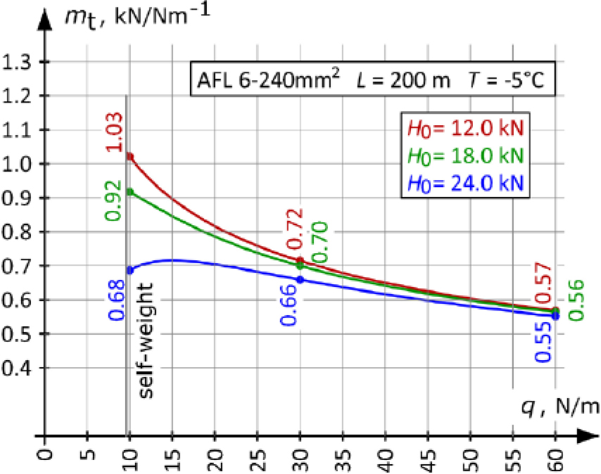
Figure 5.
The rate of tension force change mt as a function of load q for the conductor AFL-6 240 mm2
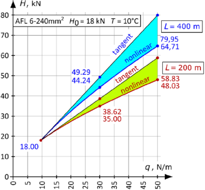
Figure 6.
Linearity deviation of the H(q) relationship for conductor AFL 6-240 mm2 in spans of 200 and 400 m
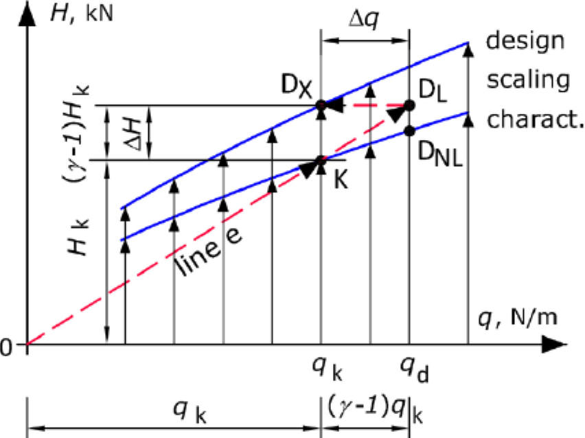
Figure 7.
Visualization of the design effects determination method
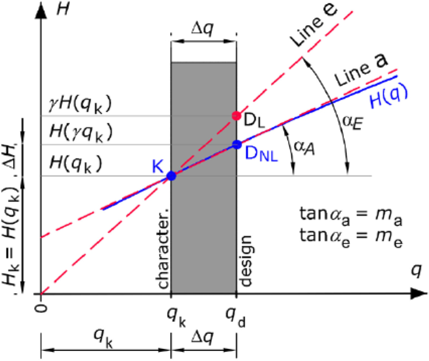
Figure 8.
Lines a and e (with slopes ma and me, respectively) used to determine the force Hd
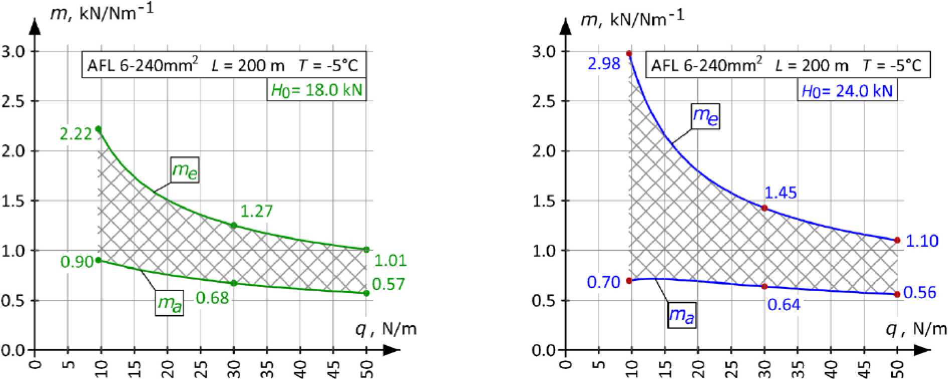
Figure 9.
Comparison of slopes ma and me for conductor AFL 6-240 mm2 (H0 = 18.0/24.0 kN)
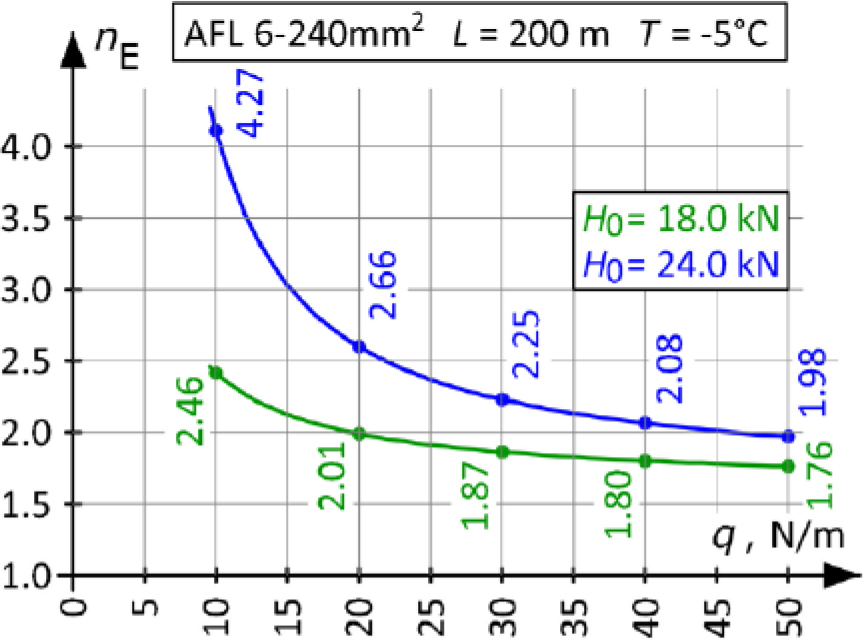
Figure 10.
Variation of the nE for AFL-6 240 mm2 conductor as a function of load (H0 = 18.0/24.0 kN)
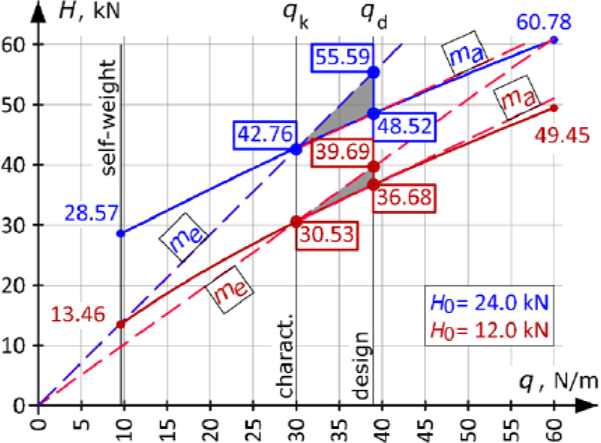
Figure 11.
Example of determining design tension forces Hd
Table 1.
Sample calculations of forces Hd and the global factor γglob,A
| 1 | 2 | 3 | 4 | 5 | 6 | 7 | 8 |
|---|---|---|---|---|---|---|---|
| qk N/m | H0 kN | Hk kN | Hd,A2 kN | Hd,A kN | Hd,E kN | nE - | γglob,A - |
| conductor AFL 6 – 240 mm2; L = 200 m; T = –5°C; γA = γE = 1.30; γG = 1.0; γI = 1.25 | |||||||
| 15.0 | 12.0 | 18.64 | 19.84 | 22.50 | 24.23 | 1.45 | 1.21 |
| 30.0 | 12.0 | 30.53 | 34.08 | 36.68 | 39.69 | 1.49 | 1.20 |
| 15.0 | 18.0 | 26.08 | 27.21 | 29.76 | 33.90 | 2.13 | 1.14 |
| 30.0 | 18.0 | 37.56 | 41.05 | 43.61 | 48.83 | 1.86 | 1.16 |
| 15.0 | 24.0 | 32.38 | 33.35 | 35.59 | 42.09 | 3.03 | 1.10 |
| 30.0 | 24.0 | 42.76 | 46.07 | 48.50 | 55.59 | 2.23 | 1.13 |
| conductor AFL 6 – 240 mm2; L = 400 m; T = –5°C; γA = γE = 1.30; γG = 1.0; γI = 1.25 | |||||||
| 15.0 | 12.0 | 18.73 | 20.25 | 23.73 | 24.35 | 1.12 | 1.27 |
| 30.0 | 12.0 | 34.67 | 39.68 | 43.40 | 45.07 | 1.19 | 1.25 |
| 15.0 | 18.0 | 27.23 | 29.09 | 33.26 | 35.40 | 1.35 | 1.22 |
| 30.0 | 18.0 | 45.85 | 51.44 | 55.54 | 59.61 | 1.42 | 1.21 |
| 15.0 | 24.0 | 34.58 | 36.48 | 40.72 | 44.95 | 1.69 | 1.18 |
| 30.0 | 24.0 | 53.48 | 59.12 | 63.25 | 69.52 | 1.64 | 1.18 |
| conductor AFL 1.7– 70 mm2; L = 200 m; T = –5°C; γA = γE = 1.30; γG = 1.0; γI = 1.25 | |||||||
| 10.0 | 10.0 | 15.98 | 17.01 | 18.19 | 20.77 | 2.17 | 1.14 |
| 20.0 | 10.0 | 22.87 | 25.24 | 26.50 | 29.73 | 1.89 | 1.16 |
| conductor AFL 1.7– 70 mm2; L = 400 m; T = –5°C; γA = γE = 1.30; γG = 1.0; γI = 1.25 | |||||||
| 10.0 | 10.0 | 18.64 | 20.37 | 22.35 | 24.23 | 1.51 | 1.20 |
| 20.0 | 10.0 | 30.05 | 33.91 | 35.95 | 39.07 | 1.53 | 1.20 |
1 Results in the columns:
1: qk – Total characteristic load of the conductor [N/m] (qk = q0 + qI),
2: H0 – Initial tension of the conductor at T = +10°C [kN],
3: Hk – Force due to the characteristic load: qk at T = −5°C [kN],
4: Hd,A2 – Force due to the design load: qd = γGq0 + γIqI (γG = 1.0; γI = 1.25) at T = −5°C [kN],
5: Hd,A – Force due to the design load: qd = γAqk (γA = 1.3) at T = −5°C [kN],
6: Hd,E – Force due to the characteristic load Hk at T = −5°C multiplied by the factor γE = 1.3,
7: nE – Ratio of the slopes of lines e and a calculated using the formula (3)
8: γglob,A – Global safety factor equal to Hd,A/Hk for the approach A.
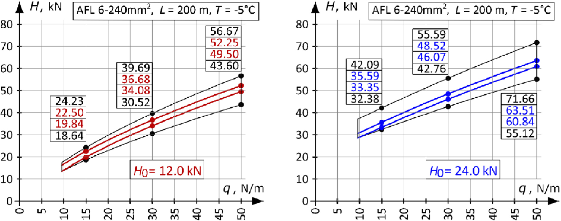
Figure 12.
Tension forces Hd according to different approaches
