A Structural Approach to Burning Number

1. Introduction

Configurations of nodes and connections emerge naturally in various applications, including physical networks (electrical circuits, street networks, organic molecules, and so on) and social networks such as Facebook. Graph theory, the branch of mathematics that studies these types of configurations, formally known as graphs, provides the fundamental framework that allows for the modeling and analysis of these networks. In return for its applications and implications on social network analysis, the mathematical product engendered by the Königsberg Bridge Problem (the problem that is often said to have been the birth of graph theory) has in recent years come out of the shadow of combinatorics to take a life of its own. Indeed, graph theory has become an invaluable contributor to understanding social networks which include groups of interacting individuals, organizations, or entities. Figure 1 depicts a Facebook network comprising 50 users (vertices) and pairwise interactions (edges) amongst them.

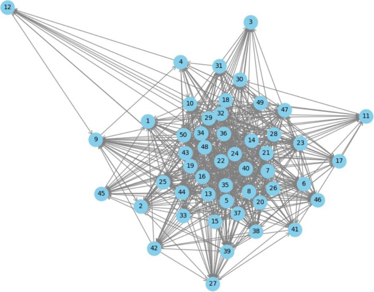
Figure 1.

Mainly due to its preeminent rise in popularity, social media has long played a dominant role in the spread of information and in the design of viral market strategies. In fact, one of the current active topics in social network analysis is the spread of social influence (Bonato, Janssen & Roshanbin 2016). According to a recent study on the spread of emotional contagion in Facebook (Kramer, Guillory & Hancock 2014), the underlying network plays an essential role as a medium for the spread of information, ideas, and influence among its members. In particular, in-person interaction and nonverbal cues are not strictly necessary for the spread. A specific example is the spread of online memes on social media platforms such as Instagram, Facebook, and X. Influence spreads from a node (an agent) to each of its neighbors (followers). Moreover, though the influence originates from a single source node, new sources of influence emerge over time in various locations in the network. Operating under these assumptions, Bonato, Janssen & Roshanbin (2016) recently proposed in a graph theoretic process called graph burning for analyzing the rate of the information spread over a network. Note that the information spread is considered as a fire spread over the network.

We now define the burning process on a finite, simple, undirected graph. Initially, all the vertices of the given graph are unburned. We then proceed to burn all the vertices in discrete time-steps or rounds. In each round, not only is a new fire started by burning a new unburned node but also all vertices adjacent to a previously burned vertex (an existing fire) will start burning as well. If a node is burned, it remains in that state until the end of the process, which is when all nodes are burned. Note that for each round, an available unburned node must be chosen as a new source of fire. Two visual illustrations of the burning process are given in Figure 2 using the same graph, known as a spider in graph theory circles. The burning source chosen in the i^th round is denoted x_i and the consecutively chosen sources of fire form what is called a burning sequence.

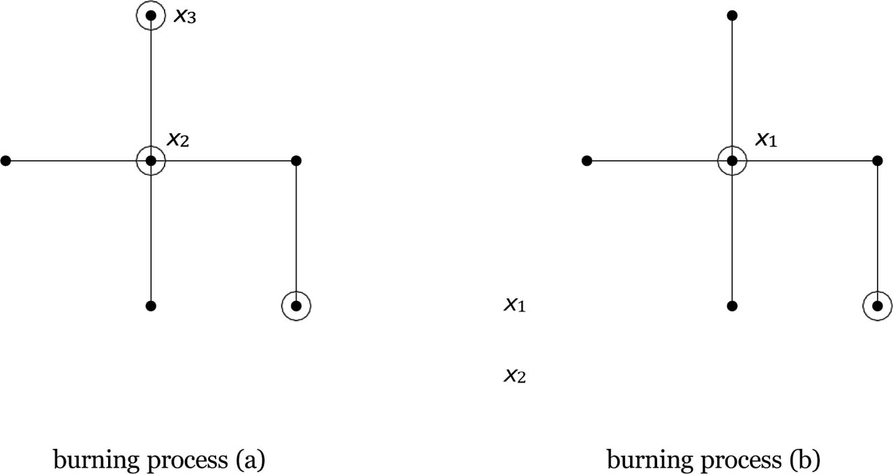
Figure 2:

These two illustrations highlight the fact that the burning process may have a lot to do with the choice of the burning sources. For example, at the end of the second round of the burning process (a), there are still three remaining nodes left to be burned, namely the pendant vertices not labeled x₁. Since a new fire must be started in each round, we choose one of these three unburned vertices to be x₃. This leads to the length of the burning sequence in (a) to be 3 while the length in (b) is 2. In fact, depending on the round in which a vertex is selected as a source, the process may be shorter or longer. Therefore, if the goal is to complete the process in the least number of rounds possible, resulting in an optimal burning sequence, then these burning sources must be strategically chosen. The burning number of a graph G, denoted b(G), is the minimum number of steps required to burn all the vertices of G. In other words, the burning number b(G) is the length of an optimal burning sequence. Equivalently, the burning number measures the optimal speed at which a graph can be burned. The lower the burning number is, the faster the fire spreads. Also, it follows immediately from the definition that for any graph with two or more vertices, the burning number is greater or equal to 2.

It is worth noting that a similar process on n-dimensional hypercubes first appeared in Alon (1992). The motivation then was a transmission problem from Intel, formulated by Alon, and they proved that the burning number of an n-dimensional hypercube is $\frac{n}{2}⌉+1$ . This process was later independently defined by Bonato, Janssen & Roshanbin (2016) and, this time, the motivation comes from the preeminent role that social networks play in spreading information (news, memes, opinions, trends, etc.) Since then, the topic of graph burning has garnered a great deal of attention, giving rise to a significant body of work. Bonato put the count at over two dozen papers in (Bonato 2021), dedicated mainly to bounding the number either in general or in the case of specific graph classes and on the computational complexity of the graph burning process. Note that the process is even NP-complete for fairly restrictive graph classes such as trees of maximum degree 3, according to Bessy et al. (2017).

In this paper, we consider a somewhat different approach to the burning number problem. More specifically, we seek to determine the kinds of graph structure(s) that are allowed under a specific burning number. To this aim, we were able to give in section 3 a characterization of all graphs with burning number 2. We then proceed to show that connected split graphs are well-burnable as well as connected {K₂ + 2K₁, P₄, C₄}-free graphs. That is, the burning number conjecture holds for these types of graphs. Lastly, in section 4, we highlight the work of an undergraduate research mentee, Tyriana Williams, in her effort to burn social media networks.

Before we can achieve these objectives, we first need some definitions and results. Also, in what follows, we consider all graphs to be non-trivial, simple, finite, and undirected, unless stated otherwise.

2. Preliminaries

In this section, we present relevant definitions, related results, and the main conjecture as well as introduce some necessary notation and terminology.

We begin with some basic definitions and terminology from graph theory. A u, v-path is a trail in a graph which does not repeat any vertex and whose endpoints are vertices u and v. The length of a path is its number of edges. The distance d(u, v) from vertex u to vertex v in G is the length of a shortest path from u to v. The eccentricity of a vertex v is defined as max{d(v, u) ∶ u ∈ V (G)}, where V(G) denotes the set of vertices of G. The radius of a graph G is the minimum eccentricity over the set of all nodes in G. The center of G consists of all nodes in G with minimum eccentricity. The diameter of a graph G is the maximum eccentricity over the set of all nodes in G. In other words, the diameter is the maximum distance between any two vertices. Also, it is not hard to see that small diameters give rise to small burning numbers. Lastly, a subset of edges that connects all vertices of G without forming any cycle (a closed path on at least three vertices) forms what is called a spanning tree of G.

Bessy et al. (2017) claimed that “burning a graph is hard.” Nevertheless, they were able to bequeath us some of the key results on the topic of graph burning, namely the following in Bonato, Janssen & Roshanbin (2016):

1. Paths play an important role in graph burning.

   Theorem 2.1. (Bonato, Janssen & Roshanbin 2016)

   Let G be a path P_n or a cycle C_n on n vertices, we have that

   $$b\left(G\right)=n^{\frac{1}{2}}⌉.$$

2. The burning number of a graph is related to other graph parameters such as its radius and diameter.

   Theorem 2.2. (Bonato, Janssen & Roshanbin 2016)

   For any graph G with radius r and diameter d, we have that

   $${\left(d+1\right)}^{\frac{1}{2}}⌉\le b\left(G\right)\le r+1$$

3. The strategy to burn the spanning tree of a graph G still works when the remaining edges in E(G) are added (i.e. Tree Reduction Theorem).

   Theorem 2.3. (Tree Reduction Theorem, Bonato, Janssen & Roshanbin 2016)

   For a graph G, we have that

   $$b\left(G\right)=min\left.b\left(T\right):T\hspace{0.17em}is\hspace{0.17em}a\hspace{0.17em}spanning\hspace{0.17em}tree\hspace{0.17em}of\hspace{0.17em}G\right\}$$

4. The relatively foremost open problem in the area of graph burning is known as the burning number conjecture, which states that

   Conjecture 2.4. (Bonato, Janssen & Roshanbin 2016)

   If G is a connected graph of order n, then

   $$b\left(G\right)\le n^{\frac{1}{2}}⌉$$

Remark that, according to theorem 2.3, proving the conjecture for trees is sufficient to prove it for any graph G. Also, if the conjecture holds, paths are then confirmed to be among connected graphs on n vertices with the largest burning number. Lastly, as a reminder, if the conjecture holds for a graph G on n vertices, the graph G is said to be well-burnable.

While the full conjecture has so far remained unresolved, it is however known to hold for special classes of graphs. For example, the conjecture is proved for various subclasses of trees, including caterpillars, trees with at most one vertex of degree at least 3, and trees without degree 2 vertices (Dhanyamol et al. 2026); so is any graph with a Hamiltonian path or cycle, which is a graph with a path or cycle that goes through each node exactly once. In such a case where the conjecture holds, we say the corresponding graph is well-burnable. In fact, as previously stated, one of the main results in this paper shows that connected split graphs and connected {K₂ + 2K₁, P₄, C₄}-free graphs are well-burnable.

A split graph is one whose vertex set can be partitioned into a clique and an independent set of vertices (Barrus & Guillaume 2022). That is, a subset of mutually adjacent vertices and a subset of mutually non-adjacent vertices, respectively. Some proper subfamilies of split graphs are well-known for their remarkable properties. For example, the threshold graphs, first defined by Chvátal and Hammer (1977), are split graphs that do not contain 2K₂, C₄, and P₄ as induced subgraphs. That is, the process of vertex deletion on a threshold graph cannot produce any of the 3 graphs listed in Figure 3: two independent edges, the cycle on four vertices, and the path on four vertices. Technically speaking, we say that threshold graphs are {2K₂, C₄, P₄}-free or the graphs listed in Figure 3 are forbidden subgraphs of threshold graphs. Note that threshold graphs can be constructed from a single vertex by repeatedly adding either an isolated vertex (a vertex that is independent of all previous vertices) or a dominating vertex (a vertex that is adjacent to all previous vertices). In general, split graphs are known to be {2K₂, C₄, C₅}-free, where C₅ denotes the cycle on five vertices.

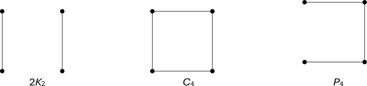
Figure 3:

Also of interest to us is another class of graphs that is known to be {K₂ + 2K₁, P₄, C₄}-free (Barrus & Guillaume 2022). In other words, graphs that do not contain any of the graphs listed in Figure 4 as induced subgraphs. They are known in Barrus & Guillaume (2022) as threshold covered graphs. In particular, we show that any connected {K₂ + 2K₁, P₄, C₄}-free graph is well-burnable. Note that {K₂ + 2K₁, P₄, C₄}-free graphs can be constructed sequentially from a 2K₂ by repeatedly adding as many dominating vertices as needed.

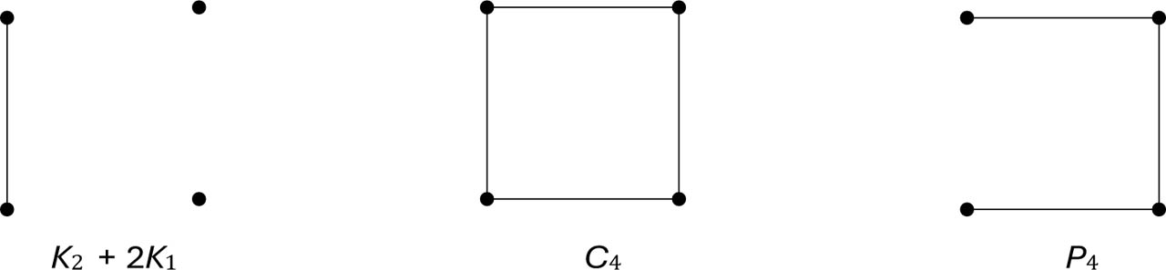
Figure 4:

We close this section by highlighting a graph parameter known to have an inverse relationship with its diameter. Commonly referred to as the graph density, it is a measure of how close a graph is to being complete, which is to being a graph in which every pair of distinct vertices is connected. Formally speaking, it is the ratio of the number of existing edges to the total number of possible edges (West 2015). Thence, we have the following duality relation between graph density and its diameter: higher density leads to lower graph diameter and vice versa.

We now proceed as follows. In the next section, we give a degree sequence characterization of all graphs with burning number 2. Then we proceed to compute the burning number of the entire class of split graphs as well as {K₂ + 2K₁, P₄, C₄}-free graphs, which are known to be non-splits since they contain 2K₂. Lastly, in section 4, we highlight the work of an undergraduate research mentee, Tyriana Williams, in her effort to burn social media networks.

3 Graph characterization & burning number of graph classes

We begin this section by establishing a necessary and sufficient condition that any graph G with b(G) = 2 must satisfy.

3. Burning social media networks

This section is dedicated to showcase some of the work performed by my undergraduate research mentee, Tyriana Williams, in the summer of 2025. The main objective was to come up with a blueprint on how to burn social media networks.

Since social network data of large platforms such as Facebook or Instagram is not available to the general public due to privacy policies, a Python program was created to randomly generate graphs that simulate the aforementioned networks. When the program runs, the user is prompted to enter how many users they want in their social network. (To access the Jupyter Notebook code, visit the GitHub repository https://github.com/JeanGuil/social-networks-graph.git.)

To evaluate the structural properties of randomly generated social media networks, the Python program was executed several times, each time with an increasing number of users in the network: 5, 10, 25, and 50. For each run, the resulting graph was visualized and analyzed. Key graph-theoretic parameters were computed, including the number of vertices, number of edges, diameter, radius, and center of the graph. The following are four distinct simulations.

4.1. 5-user social media network simulation

The simulation below corresponds to a sparse network of 5 users. The resulting graph is a low density one. Using brute force, it can be determined that the burning number of the graph is 3, which can be verified using both theorems 2.2 and 2.1. More specifically, we have that:

$$\sqrt{4+1}⌉\le b\left(G\right)\le 3\hspace{0.17em}and\hspace{0.17em}b\left(G\right)=\sqrt{5}⌉$$

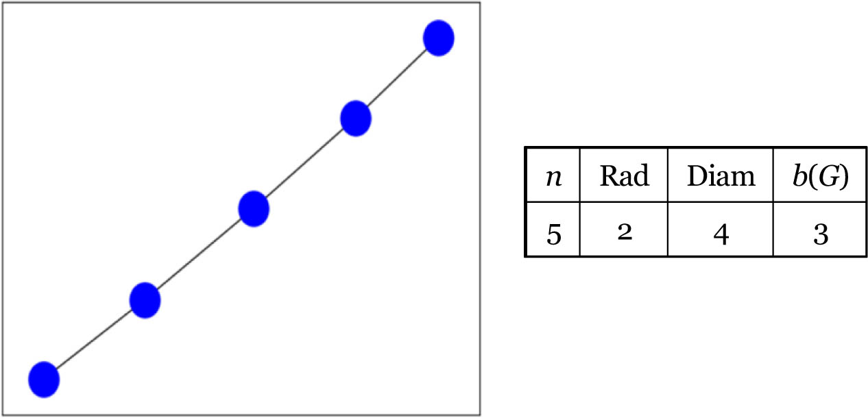
Figure 5:

4.2. 10-user social media network simulation

The simulated network below comprises 10 users. Visibly, it is less sparse and has a higher density than the previous one. Again, using brute force, it can be determined that the burning number of the graph is 3, which can be verified using theorem 2.2. More specifically, we have that:

$$\sqrt{4+1}⌉\le b\left(G\right)\le 2+1$$

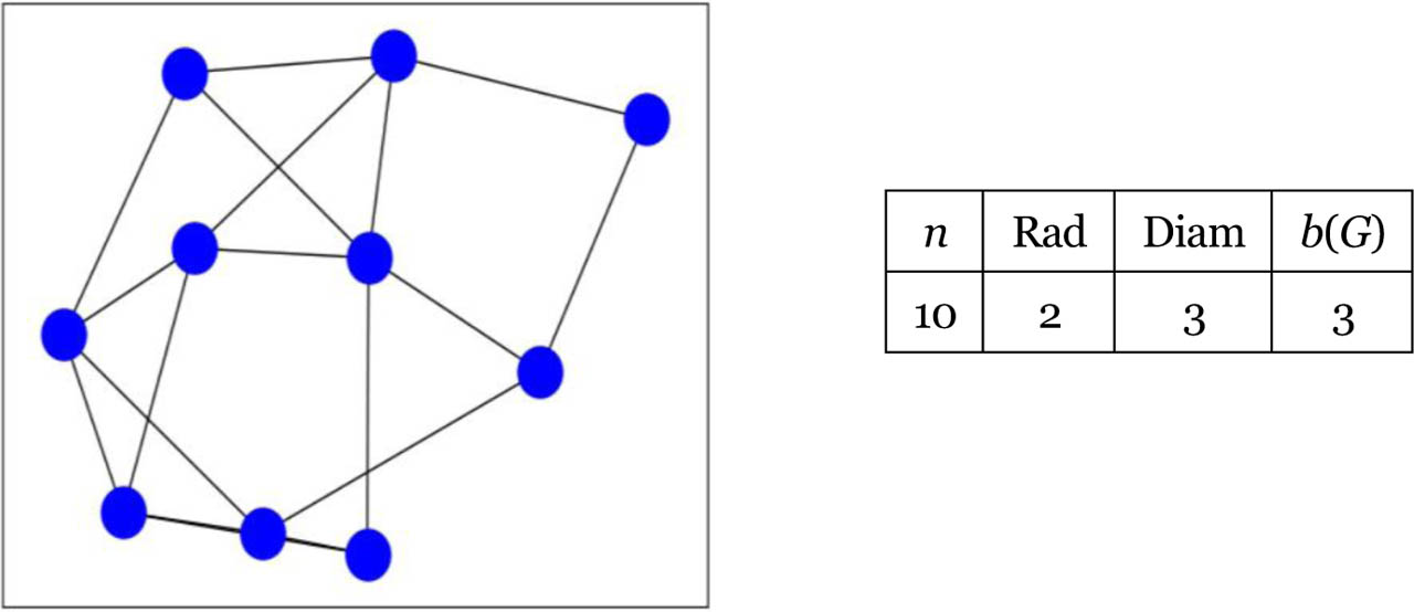
Figure 6:

4.3. 25-user social media network simulation

This time, the simulated network encompasses 25 users. The resulting graph is one with a higher density than the two previous ones. The diameter is numerically estimated at 3 and radius at 2, which leads to the burning number being less or equal to 3 by theorem 2.2.

$$\sqrt{3+1}⌉\le b\left(G\right)\le 2+1$$

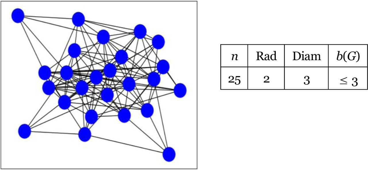
Figure 7:

4.4. 50-user social media network simulation

This final simulation corresponds to a network of 50 users. It produces a high density graph which leads to a smaller diameter and radius. Intuitively, we expect a low burning number due to the inverse relationship between density and diameter recorded in real-world networks. This is known as the small-world phenomenon where any two entities in the network are likely to be connected through a short sequence of intermediate acquaintances (Travers & Milgram 1969). Indeed, using theorem 2.2, we have that b(G) = 2.

$$\sqrt{2+1}⌉\le b\left(G\right)\le 1+1$$

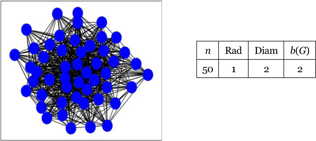
Figure 8:

In conclusion, when it comes to understanding how fast information or influence spreads within a network, we have these two main takeaways from the above simulations: 1) higher density corresponds to smaller diameter and radius, which translates into smaller burning number by theorem 2.2 and 2) an increase in connectivity translates into a decrease in burning number, hence theorem 2.3. Takeaway 1 confirms what should be an intuitive fact: highly connected social networks facilitate faster information diffusion. Equivalently, information spreads quickly and efficiently in close-knit, cohesive groups. Takeaway 2 tells however a deeper story, which is the strategy to burn a graph still works when edges are added.

5. Conclusion and future directions

In this paper, we give a necessary and sufficient condition that all graphs with burning number equal to 2 must satisfy. More specifically, we prove that, for any graph of order n, we have b(G) = 2 if and only if G has a vertex of degree at least n − 2. We successfully compute the burning number for the entire class of split graphs as well as {K₂ + 2K₁, P₄, C₄}-free graphs, which are known to be non-split since they contain 2K₂. Moreover, we prove that connected split graphs and connected {K₂ + 2K₁, P₄, C₄}-free graphs are well-burnable. Lastly, the inverse relationship between a graph connectivity and its burning number is illustrated through simulations.

Naturally, the next logical step is to characterize all graphs with burning number greater than 2. Being able to do so will also bring full resolution to long-standing related problems such as the characterization of graphs with prescribed radius, diameter, and center. To this aim, we must first remind ourselves of Bessy et al.’s (2017) warning that ”burning a graph is hard” let alone characterize all graphs of a specific burning number. By the same token, we mathematicians don’t choose to do something because it is easy. Here we go.