
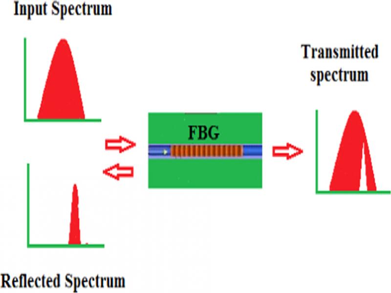
Figure 1:
Illustration of the functional principle of FBG sensors.
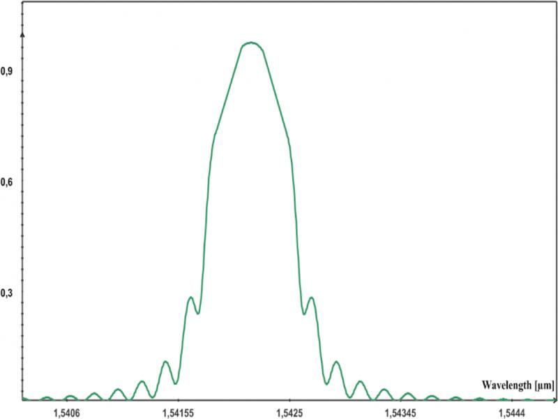
Figure 2:
Reflective spectrum of FBG sensor.
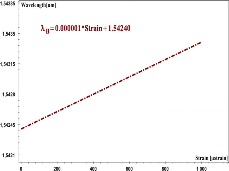
Figure 3:
Strain performance of ICFBG sensor.
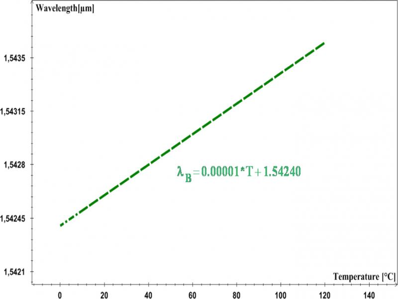
Figure 4:
Temperature performance of ICFBG sensor.
Table 1.
Examples of bridges that use the FBG technology as the basis of its SHMS.
| Bridges and country | Year | Sensors number |
|---|---|---|
| Beddington Trail, Canada | 1993 | 20 |
| Taylor, Canada | 1997 | 63 |
| Tsing Ma, China | 2003 | 40 |
| Dongying Yellow River, China | 2003 | 1,800 |
| Luiz I, Portugal | 2005 | 128 |
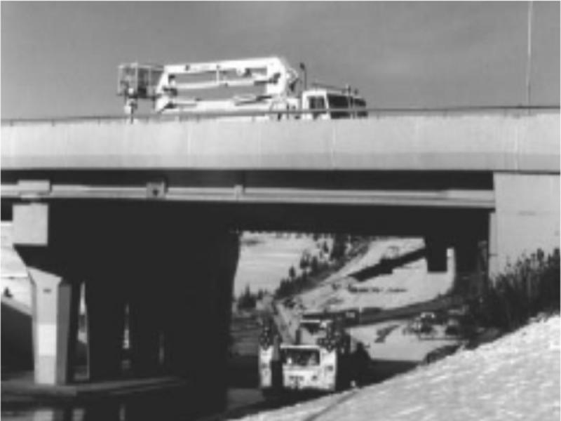
Figure 5:
The Beddington Trail Bridge in Canada (Khalil et al., 2016).
Table 2.
Examples of bridges that use fiber optic technology, and not the FBG technology, as the basis of SHMS.
| Bridges and country | Year | SHMS | Sensors number |
|---|---|---|---|
| Sungsan, South Korea | 1993 | Interferometric sensors | – |
| Versoix, Switzerland | 1998 | Low coherence sensors | 104 |
| Colle Isarco, Austria/Italy | 1999 | Low coherence sensors | 96 |
| Siggenthal, Switzerland | 2000 | Low coherence sensors | 58 |
| Götaälvbron, Sweden | 2005 | Brillouin sensors | 3 |
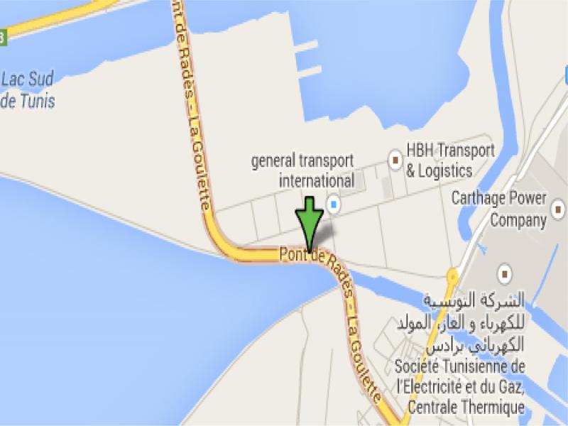
Figure 6:
Location of Rades-La Goulette Bridge in Tunisia.
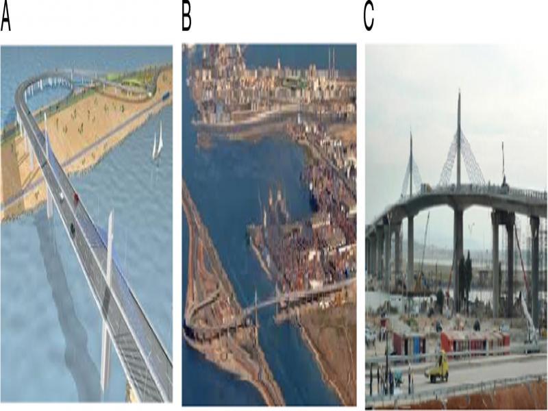
Figure 7:
General illustration of the Bridge Rades-La Goulette and their two towers (a) demonstrative model, (b) and (c) realized model.
Table 3.
The various sensors installed in the Rades-La Goulette Bridge with these measurement parameters.
| Sensor | Location | Type | Measured parameter | Number |
|---|---|---|---|---|
| Anemometer | Deck | Dynamic | Wind direction | 1 |
| Deck | Dynamic | Wind speed | 1 | |
| Load cell | Stay cables | Dynamic | Tension of cables | 12 |
| Displacement | Expansion joints | Dynamic | Movements of expansion joints | 6 |
| Low frequency accelerometers | Deck | Dynamic | Acceleration of the deck | 5 |
| Inclinometer | Towers | Static | Rotation of the towers | 4 |
| Vibrating wire strain | Concrete deck | Static | Deformation of concrete | 7 |
| Temperature | Concrete deck | Static | Concrete temperature | 14 |
| Stay cables | Static | Stay cables temperature | 2 | |
| Deck | Static | Air temperature | 1 | |
| Expansion joints | Static | Support temperature | 2 | |
| Total | 55 |
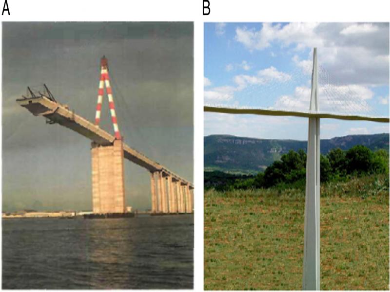
Figure 8:
Illustration of towers in (a) marine (http://www.dtrf.setra.fr) and (b) terrestrial environment (http://www.bv.transports.gouv.qc.ca).
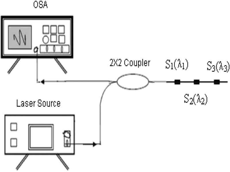
Figure 9:
Three FBG sensors network multiplexing in a single optical Fiber as SHMS for seismic effects.
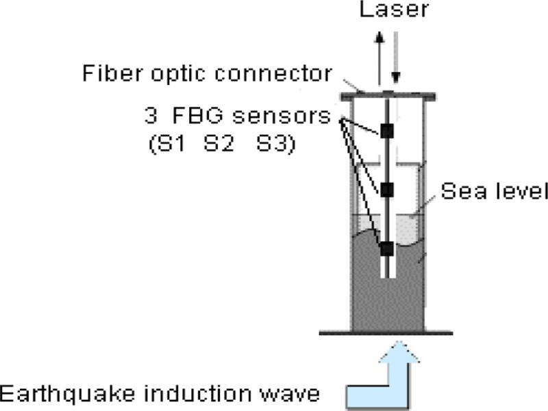
Figure 10:
Illustration of the SHMS installed into the tower to measure deflections from the vertical position due to an earthquake.
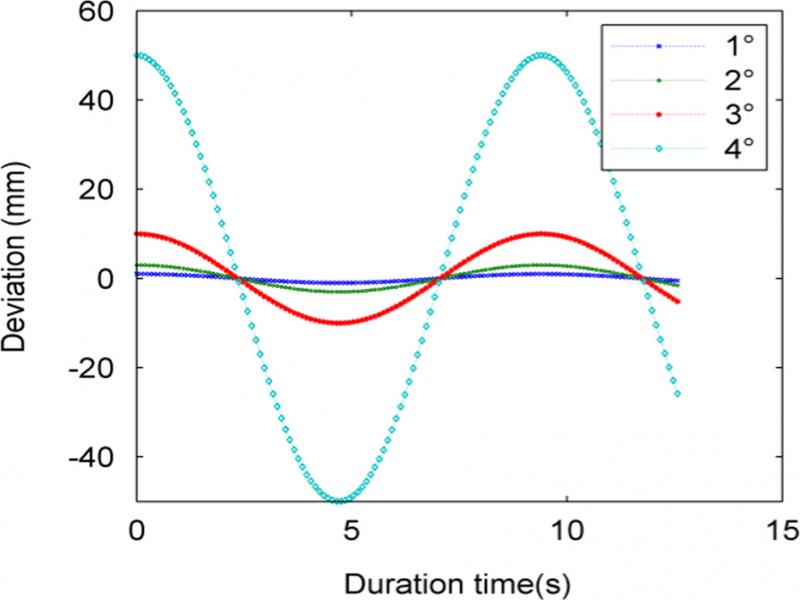
Figure 11:
Deviation response at the point where the sensor S1 is installed under seismic effects.
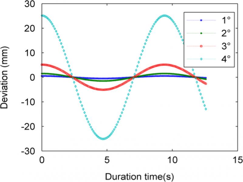
Figure 12:
Deviation response at the point where the sensor S2 is installed under seismic effects.
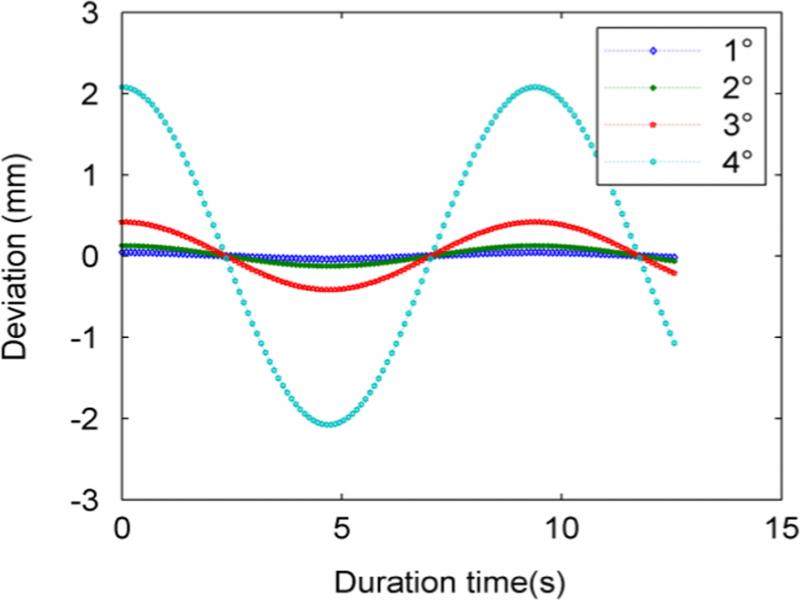
Figure 13:
Deviation response at the point where the sensor S3 is installed under seismic effects.
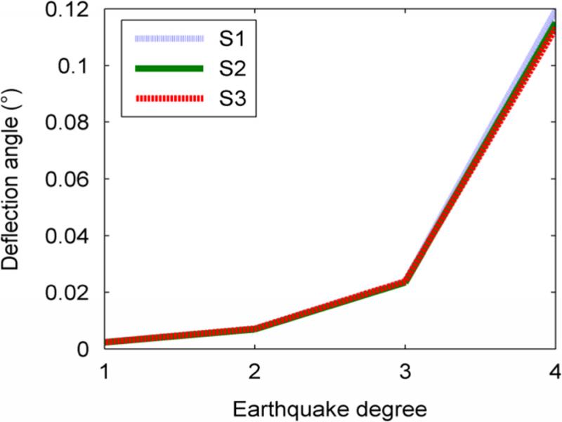
Figure 14:
Deflection angle of the tower given by the three points of reference where the sensors S1, S2, and S3 are installed in term of earthquake degree.
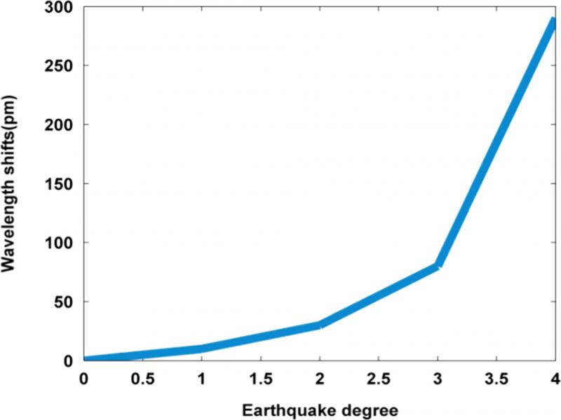
Figure 15:
Shifts of the wavelengths of the three FBG sensors network constituting the SHMS for seismic effects.
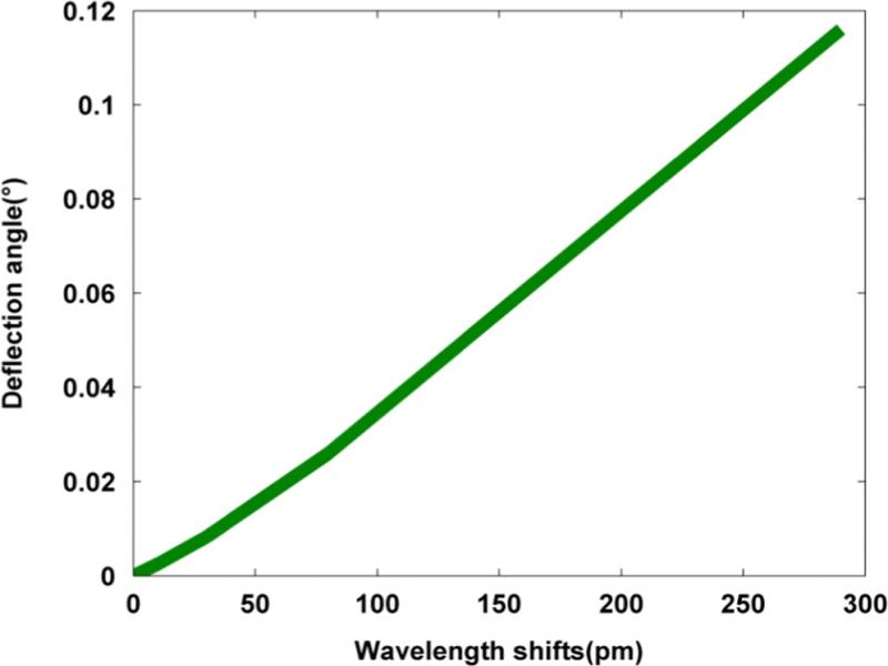
Figure 16:
The deflection angle of the tower as a function of wavelength shift of the FBG sensors constituting SHMS for seismic effects.