Development of Low Cost Autonomous Underwater Vehicle Platform

Over the years, AUVs have gained attention as specialized tools for carrying out various underwater operations, eventually leading to a dramatic increase in the number of scientific studies undertaken (Blidberg, 2001). There are four separate sub-classes of unmanaged vehicles (UVs) systems. Submersibles towed UVs behind ships are the first category, serving as ideal platforms for adding different sensors. The second category is the remotely operated vehicle (ROV), which gets directly controlled by the surface ship, with power and connectivity (Roberts, 2008). The unmanned untethered vehicle (UUV) is the third group, with its own onboard control, but is controlled remotely through a means of wireless communication protocol. Budiyono (2009). Nevertheless, the requirement for a networking link and control platform restricts ROV and UUV usage and their capability (Gonzalez, 2004). The fourth category of UVs, the AUVs, are fully autonomous underwater platforms capable of conducting underwater operations and activities and have their own sensor, control and payload equipment (Blidberg, 2001). The key benefit of an AUV is that a human operator is not required, is cheaper than a manually driven vehicle, and is able to work that is too risky for a human being (Alt, 2003; Caccia, 2006; Side and Junku, 2005; Smallwood David and Whitcomb, 2004) like monitoring of rising levels of seas (Hadi et al., 2020). In the 1980s, innovation and software developments enhanced the research to facilitate the design and implementation of sophisticated autonomous system (Blidberg, 2001). Nowadays, technicians, engineers, and computer programmers play an important role in developing technologies (Innella and Rodgers, 2021) and the developed tools can be used in various applications. The enthusiasm in AUVs in academic science has therefore been revived and several universities have built their own AUVs. The Australian Centre for Field Robotics (ACFR) of the University of Sydney runs an ocean-going AUV labeled Sirius, Designed at WHOI in the form of an Integrated Marine Observation System (IMOS), AUV facility supports competitively to facilitate deployment in Australia as a contributor to marine studies (Singh et al., 2004; Williams et al., 2009). There are many AUV contests in which a vehicle has a certain duty to carry out autonomously, which are mostly organized by colleges or other educational institutions (Gonzalez, 2004; Akhtman et al., 2008).

Power and autonomy are the two most critical technical obstacles in AUV design, since the former sets limitations on mission times and the latter decides the degree to which an AUV may be independent (Holtzhausen, 2010). While AUVs are more precise due to new technology, the creation of a completely autonomous one is an incredibly challenging problem as precise and robust controllers are required. (Salgado-Jimenez et al., 2004; Salman et al., 2011). Holtzhausen (2010) claimed that the structure of the AUV is one of the most critical aspects of an AUV. There are a number of ways to approach the construction that must take into account factors such as the pressure and/or depth needed, height, operating temperature ranges, conditions of impact, and water permeability along with corrosion and chemical resistance. The hydrodynamic coefficients that decide the dynamics of the AUV are affected not only by the structure of the AUV but also by the water current and the vehicle speed and an innovative method to evaluate velocity and heading is proposed in Rezaali and Ardalan (2016). Moreover, a hull is built to minimize the drag for reducing the propulsive force (Wang et al., 2009a). Wang stated that the first shape proposed for a hull was a spherical design, while this could withstand pressure, it influenced stability. So a circular cylindrical design, which has the benefits of being a good framework to resist the effects of hydrostatic pressure, can be expanded to provide extra room internally, seems to be a better hydrodynamic shape than a spherical one with the same volume (Ross 2006; Wang et al., 2009b). The cavitations (Kondoa and Ura, 2004) and instability (Ross, 2006) are, however, the drawbacks of a cylindrical hull. Most of the existing AUVs have a cylindrical circular hull (Evans and Nahon, 2004; Hsu et al., 2005; Woods Hole Oceanographic Institution, 2012). Similarly, a spherical shaped nose has enhanced stability and cavitation (Wang et al., 2009b).

The dynamics of an AUV are determined mainly by propulsion and buoyancy. Four kinds of propulsion systems are possible. Most common form of propulsion is via thrusters with dynamic diving technology. The other three come from static diving technology, they are piston-type ballast tank, a hydraulic pump-based ballast system and air compressor-based system (Krieg and Mohseni, 2008; Wolf, 2003).

AUV can use a single thruster for both horizontal and vertical movements with diving planes (Kondoa and Ura, 2004). The thruster technique allows the AUV to be near-neutrally buoyant with the major benefit that the vehicle can hover without propulsion. Even then, once the vehicle is in motion, the thrusters must remain ON, since it has to drive forward to remain submerged. For propulsion, most AUVs use propeller-type thrusters (Cavallo et al., 2005; Von Alt, 2003; Woods Hole Oceanographic Institution, 2012).

Jet propulsion is another method influenced by the natural locomotion of squids and other cephalopods, whereby water is pulled into a wide cavity and expelled through a nozzle at a high momentum to propel the vehicle forward (Griffiths et al., 2000). This gives the potential of an AUV to carry out low-speed maneuvering without impacting the forward drag on its structure. In this research, this type of propulsion is used to maneuver the vehicle while the propeller is being used for forward motion in the horizontal and vertical planes.

Power demands for all the equipment, such as on-board controls, motor controllers, propulsion systems, sensors and instruments, and navigation systems, must be fulfilled and supported by the electrical system of the AUV. While some AUVs are operated by fuel cells and a few uses solar power, the most popular ones are operated by batteries (Hyakudome et al., 2009; Jalbert et al., 2003). Silent operation, ease of speed regulation and simplicity are the benefits of utilizing electrical over thermal propulsion. Since lithium-ion battery technological advancements have made them an attractive alternative to silver-zinc batteries (Wilson and Bales, 2006), they are employed in our research.

A pressure sensor is the most common sensor used in vehicle depth measurement. Strain gauges and quartz crystals are the most common pressure sensor technologies for deep-ocean applications (Kinsey et al., 2006; Wang et al., 2009a).

GPS can provide superior 3-D navigation functionality. Since the water absorbs the radio signals in underwater conditions, it can be used only when a vehicle surfaces periodically to correct the readings (Nicholson and Healey, 2008). This implies that other sensors, such as the Long Baseline (LBL), Doppler Velocity Log (DVL), and magnetometer or compass are needed for the tracking and navigation of underwater vehicles for GPS fixes (Kinsey et al., 2006); e.g., Bluefin-21 AUV surfaces are needed periodically for GPS fixes. The echo sounder (Gonzalez, 2004) was used in the MAKO AUV project as another method to assess vertical depth, but only if the depth of the water is known.

The LBL, Ultra-short Baseline (USBL), and Short Baseline (SBL) systems (Kinsey et al., 2006) are known as underwater acoustic positioning systems used for depth measurement. The LBL device is essentially a method of triangulation which is used when a vehicle triangulates the acoustic position of the vehicle in the network of transponders (beacons) used on the seabed with known locations (The International Marine Contractors Association IMCA, 2009). A complete system comprises of a transceiver placed under a ship and a vehicle transponder. The time between initial acoustic pulse transmission and reaction detection is estimated and transformed into a range.

A DVL is a sensor that uses high frequency Doppler beam sonar for calculating the Doppler changes of sonar signals reflected in the ground (Wang et al., 2009b). This navigation method is only useful if the vehicle is above the sea level (18–100 m), since it is more precise at low speed and not affected by sea currents (Nicholson and Healey, 2008).

The most popular sensors used in marine equipment are magnetic sensors or electronic compass modules. Vasilijevic (Vasilijevic et al., 2012) reported that a magnetometer calculates the magnetic field of the Earth in the X, Z coordinates position and returns these three measures separately to represent the magnetic field vector values. There are a wide number of single-axis (heading only) and three-axis flux-gate magnetometers available commercially. The overall efficiency of a navigation device is mostly based on the accuracy of its magnetic sensor, which is believed to be the leading cause of error. There are three different causes of errors: the magnetic interference of the vehicle with itself or the environment (Ye et al., 2009), the compensation of the roll and pitch dependent on gravity, and finally, the orientation of the compass mounting within the vehicle.

Stutters indicated that the Inertial Navigation Device (INS) or Inertial Management Unit (IMU) utilizes accelerometers and gyroscopic sensors to detect vehicle acceleration of the three axes (Stutters et al., 2008). A gyroscope measures rotation levels, and linear acceleration is determined by an accelerometer. IMU sensors are not prone to magnetic fluctuations and drift with time, leading to erroneous measurements. Laser or fiber-optic gyroscopes do not have moving components and are included in the new INSs (Wang et al., 2009b).

A mixture of two or more of the above systems has often established some of the finest AUV navigation systems. Multi-sensor integration can be characterized as the synergistic use of multiple sensory device information that can minimize navigational errors to assist a system in carrying out its tasks (Holtzhausen, 2010).

In brief, the main objective of navigation sensors is to acquire the data and parameters of an AUV system in real time from its surrounding environment. These data are then collected by the AUV control system through its processing unit to control and maneuver AUVs effectively in order to perform a pre-identified operation.

The control accuracy provided by guidance and control systems is the basis for the successful completion of AUV missions as the autonomous control of an AUV poses serious challenges due to its complex, inherently nonlinear, and time-varying dynamics. In addition, its hydrodynamic coefficients are difficult to model accurately because of their variations under different navigational conditions and when manoeuvring in uncertain environments which expose an AUV to unpredictable external disturbances. Hence, there is a need to design and develop a robust and stable control system which can achieve AUV’s desired positions and velocities, satisfy the commands generated by its guidance system and maintain steady conditions during its mission. In order to design an adaptive controller for an AUV, suitable models of the nonlinear plant are necessary as the controllers have to cope with uncertainties due to discrepancies in modeling the unknown dynamics of the plant.

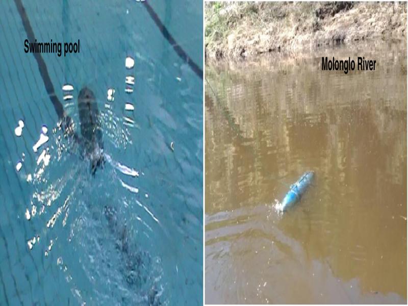
Thus, the development of an AUV for research or commercial purpose involves a number of criteria to be satisfied along with the cost. This paper proposes the development of an AUV. The main goal of this study is to develop an in-house project, find low-cost solutions for AUV navigation problems, and develop a small-sized, low-cost AUV. The platform is expected to demonstrate autonomous manoeuvre for changing conditions and under the influence of external disturbances in a controlled environment such as a swimming pool.

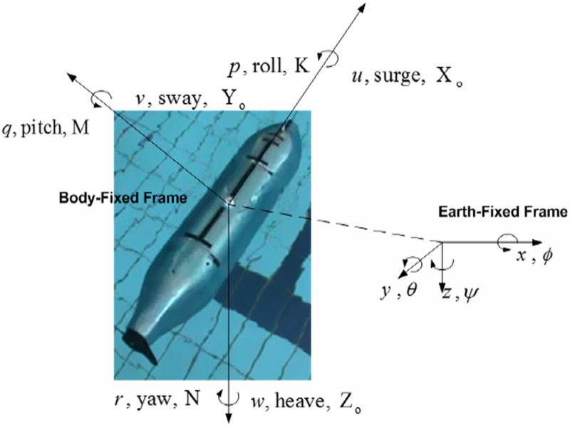
The rest of the paper structure is organized as follows. The detailed specifications of different AUV subsystems considered for the work in this study are described in the second section. The third section discusses the AUV complete system and its integration. The kinematics and the nonlinear mathematical modeling of an AUV in 6-DOF is discussed in the fourth section that includes the Simulink/Matlab model of the AUV along with the investigation of its open-loop characteristics. The main features of the Hardware-in-Loop (HIL) simulation are explained in the fifth section. The sixth section presents the experimental results of the proposed model-based control algorithm on the AUV. The study is concluded in the final section.

Platform design

The integration on the UNSW Canberra AUV with electrical and electronic systems, which include prototypes, specifications, power distribution system and storage, actuators and sensors, is discussed. The instrumentation required to accommodate on board the AUV in order the completely collect the data associated with different maneauvers, the interface and integration of all subsystems with the PC 104 device are addressed.

This paper presents the development of an AUV experimental platform with adaptive control capabilities aimed at achieving the mission requirements. A detailed block diagram indicating different stages in this project is shown in Fig. 1.

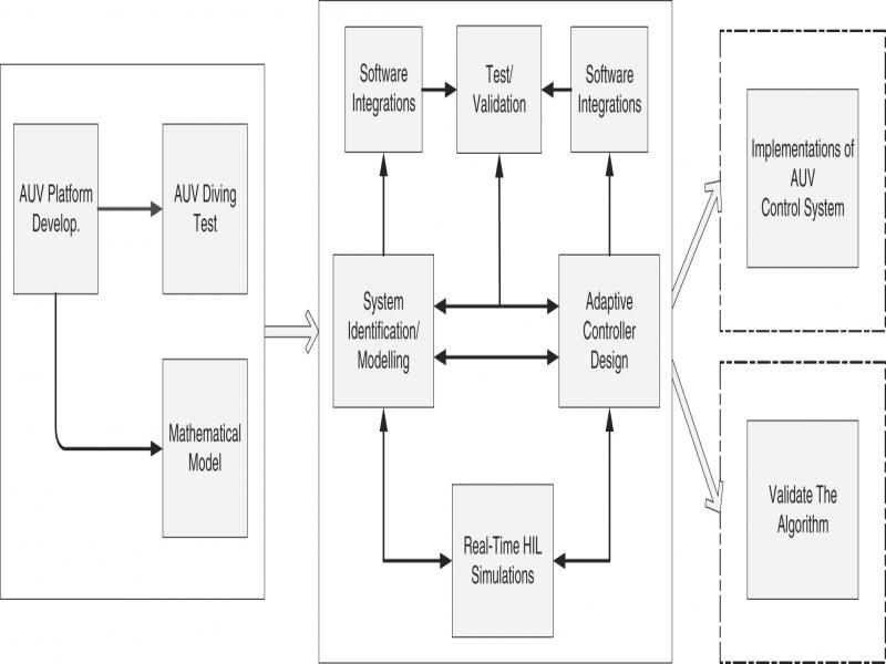
Figure 1:

UNSW Canberra AUV platform

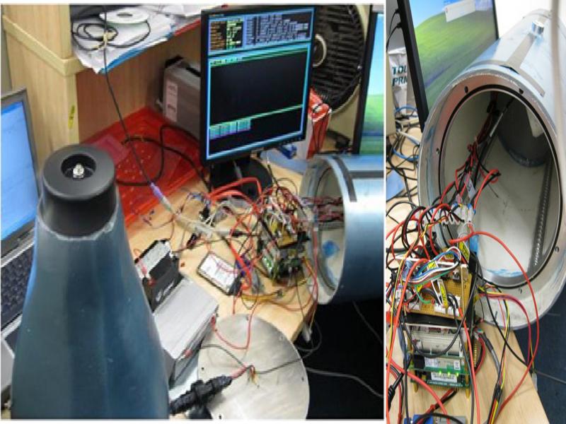
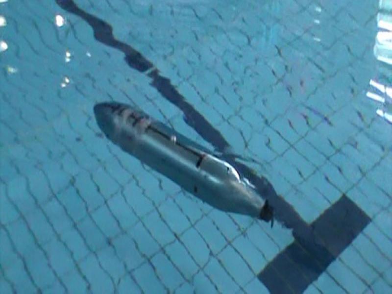
In the UNSW Canberra workshop, a torpedo-shaped underwater vehicle prototype is constructed as a demonstration of the concepts of the underwater vehicle, which comprises of three segments; nose cone, body (middle section), and tail cone. Hassanein et al. (2011, 2013). The nose and tail cone moulds are made up of Stayfoam, then wrapped with fiberglass and those are wet sections to decrease the buoyancy force. The body is made of a 255 mm PVC pipe and is known to be the dry section where the batteries are located along with the circuitry, sensors, and control unit. The dry portion is segregated by the bulkheads for providing waterproof environment. An on-board data logger and control unit have been equipped with the AUV platform to allow sensor and actuator data to be recorded and processed to implement advanced system identification and control techniques. Necessary computers and sensors are chosen, considering the need for low cost, compact, simplicity of program and processor capabilities. The UNSW Canberra AUV model is shown in Fig. 2.

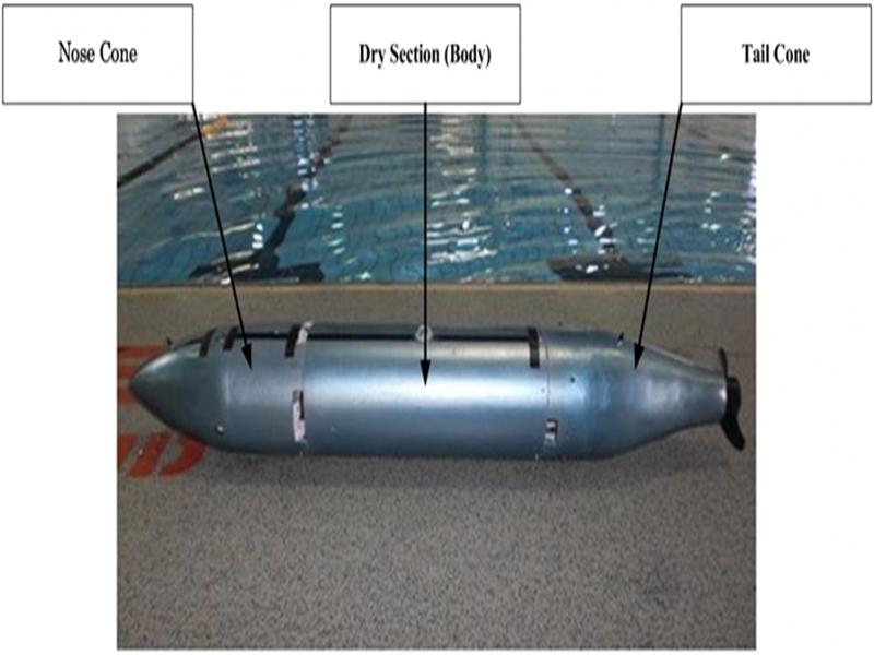
Figure 2:

Actuators

The AUV employs two forms of actuators, the electrical propeller for thrust and secondly, four bilge pumps to operate in the horizontal and vertical axis.

The thrusters that use propeller systems and a small DC motor wrapped in a watertight enclosure to spin the propeller that produce torque are the key method of actuation in the AUV. The existing thruster is a 12Vdc electric motor, typically employed for small river vessels. The ‘Endura C2’ thruster was obtained from a ‘MINN KOTA’ company shown in Fig. 3. An ‘ET-OPTO RELAY4’ made by the ‘ETT’ company is used since the electric motor requires a controller or driver shown in Fig. 3. According to the function and operating order, this has two inputs to drive the motor, the power given by the battery and a control signal from the I/O module in the processor unit.

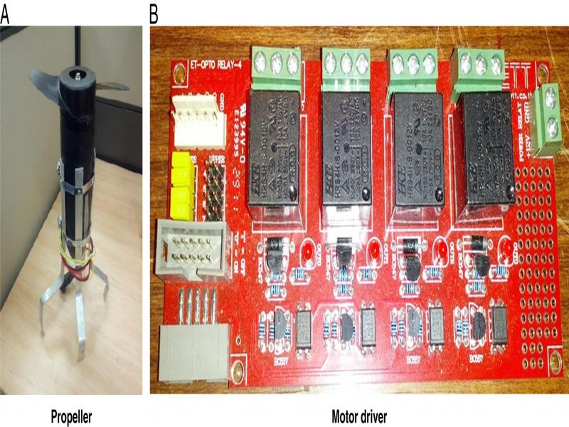
Figure 3:

In order to maneuver in horizontal and vertical planes (pitch and lake angle), submersible bilge pumps are obtained from a company named ‘Rule Mate.’ These are shown in Fig. 4. There are three distinct pump configurations and all the pumps are battery operated by 12 Vdc. The left and right pumps used to control the AUV in the horizontal plane have an output of 750 GPH and a force of 0.0022 N. The pump used to push down this vehicle is rated by 0.0033 N at 1,000 GPH and by 0.0044 N at 1,500 GPH. The pumps are operated in on/off mode using the control unit’s PWM signals. The motor driver for such pumps is an ET-OPTO DC-OUT4 manufactured by ETT as shown in Fig. 4.

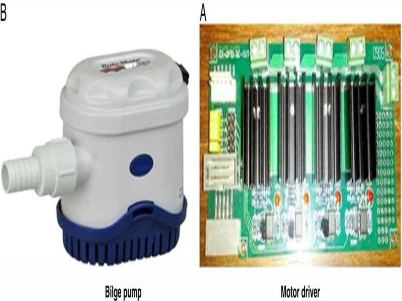
Figure 4:

Inertial measurements UNIT (IMU)

The IMU is the key sensor used for AUV navigation and comprises three gyroscopes and three accelerometers, each mounted along the X, Y, and Z axes for the calculation of rotational speeds and linear accelerations. The gyroscope data was used to calculate the rotations of the vehicle along the three axes indicated by roll, pitch, and yaw. In terms of these three DOFs, the rotational position of the vehicle is calculated by the determination of the rotational velocity integral over the period of the measurement. In order to determine the location of the vehicle in a three-dimensional space, one must continuously convert from the local coordination system of the vehicle to the coordination system of the earth. This transformation is addressed later in this paper. The ADIS16367 shown in Fig. 5 is the unique IMU used in this project, which is a 3-axis system acquired from Analog Devices Co. The ADIS16367 combines industry-leading and signal conditioning IMEMS technology that optimizes dynamic efficiency and is a comparatively cheap device. IMU outputs are compared with the calibrated digital compass outputs with no major errors amongst them.

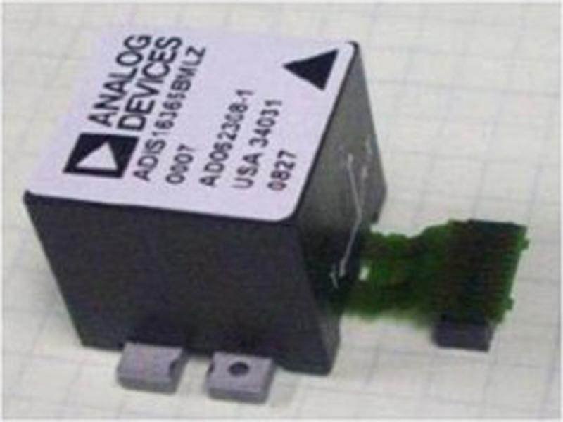
Figure 5:

A serial peripheral interface (SPI) card was designed and developed as part of this project as shown in Fig. 6. An I/O board is necessary for dealing with the lower level interface between the IMU and the processing device. The I/O module is on the ATmega168-based Arduino Pro-Mini microcontroller board consisting of 14 digital input/output pins, 6 analog inputs, an on-board resonator, a reset button and pin header mounting holes. To provide communication to the board and USB power, a six-pin header can be plugged into an FTDI cable or Sparkfun breakout board. The serial peripheral interface sends the data to the PC104 at a rate of 115 kbps through an RS232 serial port.

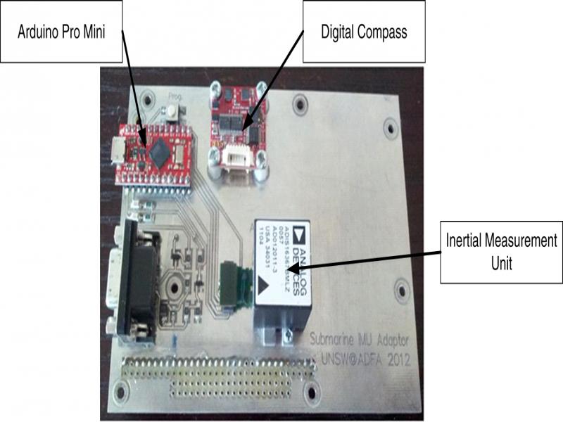
Figure 6:

A ‘burst data read collection’ is the best way to retrieve data from the IMU, which is a process-efficient form of obtaining ADIS16367 data in which all output registers are clocked on DOUT (SPI Data Output), 16 bits at a time, in sequential data cycles (each divided by a single SCLK interval (SPI Serial Clock)). DIN (SPI data input) is set to 0x3E00 to start a burst read sequence, then the contents of every output register is transferred to DOUT, that is from SUPPLY OUT to AUX ADC, as seen in Figs. 6 and 7. The data are being sent to a PC104 on-board COM port which contains RS232 driver blocks to handle serial communications provided by the Matlab xPC goal toolbox.

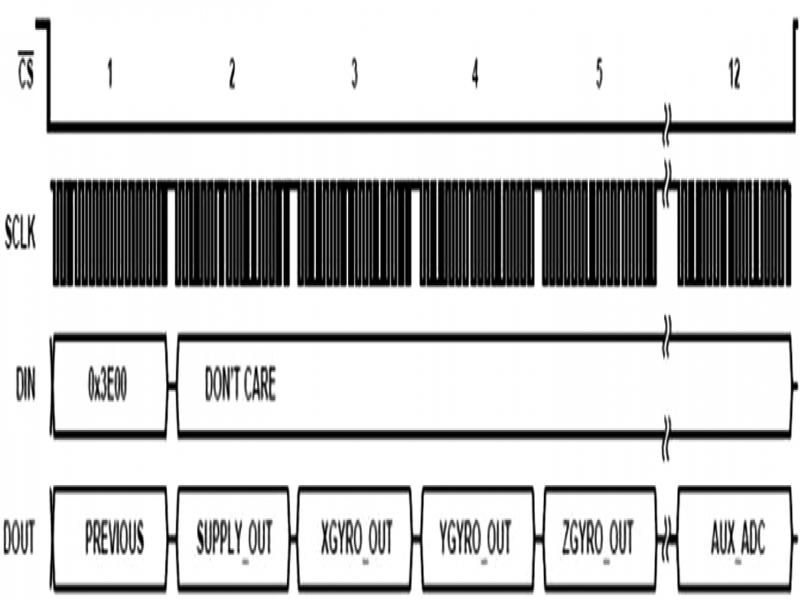
Figure 7:

Electronic Digital Compass

A magnetometer or electronic digital compass is also a sensor used for the AUV navigation, which measures the magnet field of the Earth in the direction of the X, Y, and Z axes. It returns the three measurements separately to provide the magnetic field vector values, which are then used for determining the heading of the vehicle. It does not need to be transformed since this heading calculation is taken in the global reference frame or coordinates. The magnetometer is susceptible to other disturbance in the magnetic field of the Earth. To stop incorrect readings, it can be recalibrated before any dive. The magnetometer can often be disturbed by other magnetic objects in close vicinity of the sensor as well.

As shown in the Fig. 8, an Oceansever OS5000-USD with a depth sensor, a 3-axis tilt-compensated compass with both Serial & USB direct interfaces and connections on both sides of the module, is the digital compass used in this project. It comprises a 3-axis AMR magnetic tracker, a 3-axis STM accelerometer, a 50 MIPS microprocessor that facilitates precise tilt correction floating point IEEE operations and 24-bit differential input Sigma-Delta AD converters.

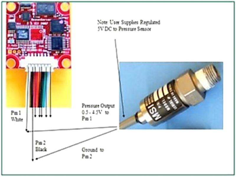
Figure 8:

For operation, the compass needs power supply of 5 V, when attached to the pressure sensor, it measures the depth and its outputs include a heading, pitch and roll in degrees, a 3-axis magnetic field, a 3-axis acceleration, gyro reading in 2 axes and temperature. Its built-in calibration involves rotation around the Z, Y, and X axes that takes place after installation in the AUV and before the experiments begin.

Water pressure sensor

The water pressure is a variation in the surface pressure and it is calculated in Pascals (Pa). A water pressure sensor used in this project for measuring the water pressure on the exterior of the vehicle and for determining the vehicle’s depth. As there is a linear relationship between the water pressure and the vehicle’s depth, this can be easily determined from Pascals law,

(1)

$$\Delta P=\rho g(\Delta h),$$

(1)where ρ is the water density in kg/m3, Δh is the depth of the vehicle in meters (m) and g is the gravitational acceleration (9.81 m/s²).

The water pressure sensor used in this project is an LM series low-pressure media-isolated sensor with an analogue interface. It uses three wires, power, ground and signal. The output signal range is between 0.5 and 4.5 V depending on the pressure. The relationship between the measured voltage and water pressure is linear. As this sensor has a measuring range from 0 to 15 PSI, it can be used to measure depths of up to 10 m. It is connected directly to the digital compass to calculate the depth, as shown in Fig. 8.

A 50 cm tube with a tape measure is placed on the sensor to calibrate the sensor. The water is then fed into the tube every 2 cm and the values obtained were recorded. The error of depth measurement is less than 0.14 mm. Fig. 9 shows the acquired precision of the measurement.

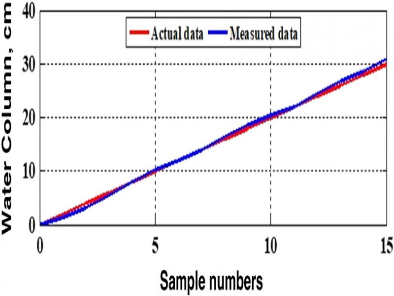
Figure 9:

On-board computer

AUV is managed by an on-board processing unit, which involves fast processors and broad memories. The PC104 architecture is one of those widely used processors for embedded systems. A great feature of the architecture of the PC104 is that it has a defined form factor that enables to have several add-on boards compatible with the main processor card. The other benefits of the PC104 system are its compact size and high processing capacity. There is an Industry Standard Architecture (ISA) bus for these PC104 boards that runs through all the interconnected boards. On the ISA bus there are 104 pins. The PC104-plus comes with an ISA bus and a peripheral part interface (PCI). The PCI bus works at lower levels of voltage and is much faster than the ISA bus. In contrast to the ISA bus width of 16 bits, the PCI bus is 32 bits or 64 bits wide.

Compared to many other architectures, the advantages of a PC 104-based embedded device have contributed to the usage of this AUV design in UNSW Canberra with a PC104-plus, which comprise the core of the AUV control unit. It incorporates an Intel Atom N450 processor with 1 GB RAM, 250 GB hard drive, speed of 1.66 GHz, and it uses a compact flash disk for real-time applications as data storage.

It consists four USB ports, one Ethernet port and two serial COM ports. The serial ports are either RS-232 or RS-485, chosen by jumpers on the chip-set. Fig. 10 shows the analog and digital I/O boards and a DC-DC supply card; these are also included in the modules on the PC104 Stack.

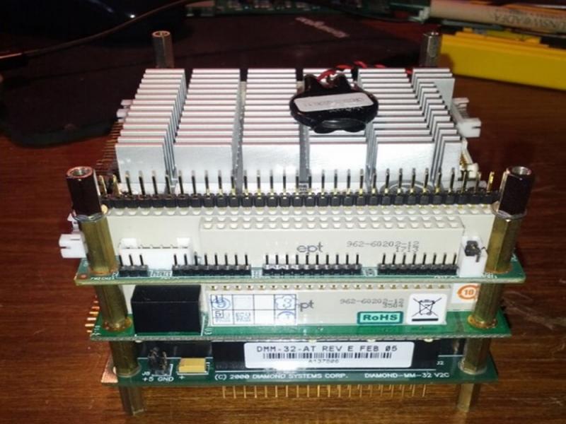
Figure 10:

The dedicated PC104 architecture power supply board PCM-3910, is used to provide constant voltages of various amplitudes. As compared to other standard methods, this board provides reliable voltage regulation. This board has a 10–30 V input range and provides on-board 5, 12, ‒5, and ‒12 V outputs for the stack and various sensors. PC104 stack also contains an Analog-to-Digital (A/D) conversion board, DMM-32X-AT by Diamond Systems. The resolution of A/D is 16-bit with 32 analog channels.

The PC104’s real-time environment is an xPC target, a Matlab toolbox that offers the Matlab® Simulink® real-time kernel and application development environment. It instantly produces code via the Real-Time Workshop (RTW), which can be downloaded to a second computer utilizing the xPC target real-time kernel for simplification and minimization of development time and debugging. Using the Simulink® libraries available on Matlab®, the Simulink model is initially developed and then compiled using the xPC target option which creates an executable embedded code that can be downloaded to the target device.

System integration

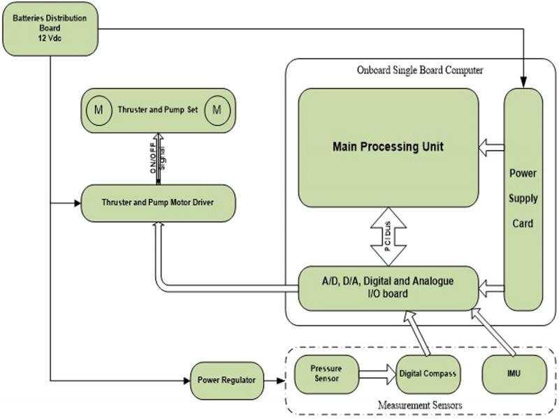
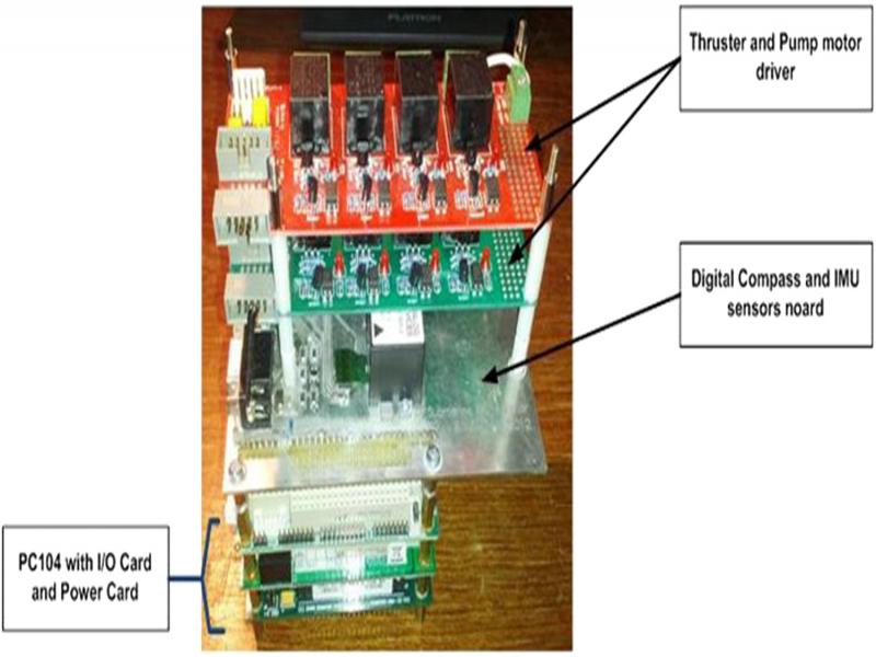
The PC104 is the system that performs all of the key control tasks. It is then link to the IO module, which includes low-level interfaces for both sensors and actuators. Fig. 11 displays the whole system and its integration, showing all interfaces between the AUV hardware and component interfaces. The integrated system used to control the AUV maneuvering is shown in Fig. 12. Eventually, the AUV parameter values are measured and indicated in Table 1 (Hassanein et al., 2013).

Table 1.

Specifications of AUV model.

Figure 11:

Figure 12:

Buoyancy would be a problem that requires a lot of consideration in order to submerge the vehicle. The power supply along with the power distribution system, actuators and other instruments, all sensors, and PC104 computer are located in the dry section of the vehicle. Initially, the entire vehicle was placed in the water, a strap test rig is wrapped around the vehicle and a hanger is then added to carry weights. This allows one to add weight until the buoyancy of the vehicle is resolved, enabling one to see how much weight is needed in the vehicle. By taking into consideration of the gravity and buoyancy centers, this weight is placed in the dry area. In addition, the nose and tail cones are equipped with an air tube in order to fine-tune the vehicle’s buoyancy at the start of each examination. The neutral vehicle buoyancy in the UNSW Canberra swimming pool is shown in Fig. 13.

Figure 13:

AUV dynamic modeling

The AUVs is modeled via the analysis of statics and dynamics. The first is for the equilibrium of a body at rest or moving at constant speed and the second is the body experiencing accelerated movement (Hassanein et al., 2011, 2013). The coordinate system and specifications of the motion parameters should be given first in order to derive a 6-DOF nonlinear mathematical model of the AUV.

Coordinate system

The position, orientation, linear velocity, and angular velocity of an underwater vehicle are defined in two frames of reference. The first frame is the X_OY_OZ_O fixed frame, typically chosen to match the body’s CG and represented in relation to a gravitational reference or the Earth-set frame, E-xyz as seen in Fig. 14. As with underwater vehicles, it is believed that the acceleration of a position on the surface of the Earth may be ignored (Hassanein et al., 2013), the Earth-fixed frame is known to be inertial in this work. The position of the vehicle and its orientation in relation to the inertial reference frame, and linear and angular velocities are described to be the body reference frame. The typical evaluations for SNAME (1950) underwater vehicles as described on Nomenclature appendix (Antonelli, 2018; Antonelli et al., 2008; Fossen, 1994; Hassanein et al., 2011, 2013).

Figure 14:

Kinematics

The position and orientation of the vehicle, as mentioned earlier, is defined with regard to the inertial reference system in which ${\eta }_1\in {\Re }^3$ determines the position of the body (Antonelli, 2018; Antonelli et al., 2008),

(2)

$${\eta }_1=[\begin{array}{c}x\\ y\\ z\end{array}],$$

(2)where the vector ${\dot{\eta }}_1$ is the corresponding derivative time and is also connected to the inertial frame as (Antonelli, 2018; Antonelli et al., 2008),

(3)

$${\nu }_1=[\begin{array}{c}u\\ v\\ w\end{array}],$$

(3)where ${\nu }_1$ is the linear velocity of the body-fixed frame of origin, which can be defined as the body-fixed frame with regard to the inertial reference frame (Antonelli, 2018; Antonelli et al., 2008),

(4)

$$R_I^B=[\begin{array}{ccc}{c}_{\psi }{c}_{\theta }& s_{\psi }{c}_{\theta }& -s_{\theta }\\ -s_{\psi }{c}_{\phi }+c_{\psi }{s}_{\theta }{s}_{\phi }& c_{\psi }{c}_{\phi }+s_{\psi }{s}_{\theta }{s}_{\phi }& s_{\phi }{c}_{\theta }\\ s_{\psi }{s}_{\phi }+c_{\psi }{s}_{\theta }{c}_{\phi }& s_{\psi }{s}_{\phi }+s_{\psi }{s}_{\theta }{c}_{\phi }& c_{\phi }{c}_{\theta }\end{array}],$$

(4)where $R_I^B$ is the rotational matrix that describes the inertial frame transformation and can be described as the fixed frame,

(5)

$$R_I^B=[\begin{array}{ccc}{c}_{\psi }{c}_{\theta }& s_{\psi }{c}_{\theta }& ‒s_{\theta }\\ ‒s_{\psi }{c}_{\phi }+c_{\psi }{s}_{\theta }{s}_{\phi }& c_{\psi }{c}_{\phi }+s_{\psi }{s}_{\theta }{s}_{\phi }& s_{\phi }{c}_{\theta }\\ s_{\psi }{s}_{\phi }+c_{\psi }{s}_{\theta }{c}_{\phi }& s_{\psi }{s}_{\phi }+s_{\psi }{s}_{\theta }{c}_{\phi }& c_{\phi }{c}_{\theta }\end{array}],$$

(5)where $c_{\theta }\mathrm{and}{s}_{\theta }$ are short notations for $\cos \theta \mathrm{and}\sin \theta$, respectively. Similarly, to define the underwater vehicle orientation, ${\eta }_2\in {\Re }^3$ is described by the body’s co-ordinates in the inertial frame (Antonelli et al., 2008; Hassanein et al., 2011),

(6)

$${\eta }_2=[\begin{array}{c}\phi \\ \theta \\ \psi \end{array}],$$

(6)where ${\eta }_2$ is the body Euler-angle coordinates in the inertial frame, commonly called roll, pitch and yaw, respectively,

(7)

$${\nu }_2=[\begin{array}{c}p\\ q\\ r\end{array}],$$

(7)where ${\nu }_2$ is the angular velocity vector of the origin of the body-fixed frame in order to attain that, with respect to the inertial frame of reference described in the body-fixed frame,

(8)

$${\nu }_2=J_1({\eta }_2){\dot{\eta }}_2,$$

(8)where the vector describing the angular velocity of the body-fixed frame relative to the inertial frame is ${\nu }_2$. It must be observed that the ${\dot{\eta }}_2$ vector has no physical significance and its relationship to the body-fixed frame is through the proper Jacobian matrix $J_1$, and the Jacobian matrix $J_1\in {\Re }^{3{\rm X}3}$, is within the Euler angles expressed as,

(9)

$$J_1({\eta }_2)=[\begin{array}{ccc}1& 0& ‒\sin \theta \\ 0& \cos \theta & \cos \theta \sin \phi \\ 0& ‒\sin \phi & \cos \theta \cos \phi \end{array}].$$

Equations of motion

Equations of Motion for a rigid body can be obtained from Newton’s second law and a rigid body’s dynamic behavior is generally written in the notation of SNAME (1950) as described on Nomenclature appendix (Antonelli, 2018; Antonelli et al., 2008; Fossen, 1994; Hassanein et al., 2011, 2013). The rigid body dynamics can be written in component form as:

• For translational motion:

  $$X=m[\dot{u}‒vr+wq‒x_G(q^2+r^2)+y_G(pq‒\dot{r})+z_G(pr+\dot{q})]$$
  $$Y=m[\dot{v}-wp+ur‒y_G(r^2+p^2)+z_G(qr‒\dot{p})+x_G(qp+\dot{r})]$$
  $$Z=m[\dot{w}‒uq+vp‒z_G(p^2+q^2)+x_G(rp‒\dot{q})+y_G(rq+\dot{p})]$$

• For the rotational motion

(10)

$$\begin{array}{c}K=I_x\dot{p}+(I_z‒I_y)qr‒(\dot{r}+pq)I_{xz}+(r^2‒q^2)I_{yz}+(pr‒\dot{q})I_{xy}\\ +m[y_G(\dot{w}‒uq+vp)‒z_G(\dot{v}‒wp+ur)]\\ M=I_y\dot{q}+(I_x‒I_z)rp‒(\dot{q}+qr)I_{yz}+(p^2‒r^2)I_{zx}+(qp‒\dot{r})I_{yz}\\ +m[z_G(\dot{u}‒vr+wq)‒x_G(\dot{w}‒uq+vp)]\\ N=I_z\dot{r}+(I_y‒I_x)pq‒(\dot{q}+rp)I_{yz}+(q^2‒p^2)I_{xy}+(rq‒\dot{p})I_{zx}\\ +m[x_G(\dot{v}-wp+ur)‒y_G(\dot{u}-vr+wq)]\end{array}$$

The above equations represented in a compact form as,

(11)

$$M_{RB}\dot{\nu }+C_{RB}(\nu )\nu ={\tau }_{RB}$$

where $M_{RB}$ is the rigid-body inertia matrix and $C_{RB}$ the rigid-body Coriolis and Centripetal matrix.

Property 3.1 The parameterization of $M_{RB}$ is unique and satisfies,

(12)

$$M_{RB}=M_{RB}^T>0;{\dot{M}}_{RB}=0$$

(13)

$$M_{RB}=[\begin{array}{cccccc}m& 0& 0& 0& m{z}_G& ‒m{y}_G\\ 0& m& 0& ‒m{z}_G& 0& m{x}_G\\ 0& 0& m& m{y}_G& ‒m{x}_G& 0\\ 0& ‒m{z}_G& m{y}_G& I_x& ‒I_{yx}& ‒I_{xz}\\ m{z}_G& 0& ‒m{x}_G& ‒I_{yx}& I_y& ‒I_{yz}\\ ‒m{y}_G& m{x}_G& 0& ‒I_{zx}& ‒I_{zy}& I_z\end{array}]$$

Property 3.2, $C_{RB}$ can always be parameterized such that it is skew-symmetrical, that is,

(14)

$$C_{RB}(v)=‒C_{RB}^T(v)\forall \nu \in {\Re }^6$$

$$C_{RB}=[\begin{array}{ccc}0& 0& 0\\ 0& 0& 0\\ 0& 0& 0\\ ‒m(y_{G}q+z_{G}r)& m(y_{G}p+w)& m(z_{G}p‒v)\\ m(x_{G}q‒w)& ‒m(y_{G}q+z_{G}r)& ‒m(y_{G}q+z_{G}r)\\ ‒m(y_{G}q+z_{G}r)& ‒m(y_{G}q+z_{G}r)& ‒m(y_{G}q+z_{G}r)\end{array}$$

(15)

$$\begin{array}{ccc}‒m(y_{G}q+z_{G}r)& ‒m(y_{G}q+z_{G}r)& ‒m(y_{G}q+z_{G}r)\\ ‒m(y_{G}q+z_{G}r)& ‒m(y_{G}q+z_{G}r)& ‒m(y_{G}q+z_{G}r)\\ ‒m(y_{G}q+z_{G}r)& ‒m(y_{G}q+z_{G}r)& ‒m(y_{G}q+z_{G}r)\\ 0& I_{yz}q+I_{xz}p‒I_{z}r& I_{yz}q+I_{xz}p‒I_{z}r\\ I_{yz}q+I_{xz}p‒I_{z}r& 0& I_{yz}q+I_{xz}p‒I_{z}r\\ I_{yz}q+I_{xz}p‒I_{z}r& I_{yz}q+I_{xz}p‒I_{z}r& 0\end{array}]$$

An underwater vehicle’s general equation of motion can be written as (Hassanein et al., 2011),

(16)

$$M_{RB}\dot{v}+C_{RB}(v)v+M_A\dot{v}+C_A(v)v+D(v)v+g(\eta )=\tau$$

(16)where $\tau$ vector of control inputs. The terminology of the rigid-body describe the rigid body’s equation of motion in an empty space. Nevertheless, hydrodynamic theories have been applied to the equation because ships and underwater vehicles require the presence of accelerations caused by fluid to be taken in to account, whereas hydrostatic concepts reflect the gravitational force and buoyancy that exist while a rigid body is completely or partially immersed in a fluid. The added mass and inertia and damping effects compose the hydrodynamic terms.

The added inertia of the fluid around the body is accelerated by the motion of the body which must be included in the equations of motion when a rigid body is submerged which travels in a fluid. Fossen has stated that, as the air density is significantly lower than that of a moving mechanical system, it is possible to ignore the impact of the additional mass and inertia in industrial robotics (Fossen, 1994). In the case of an underwater vehicle application, the water and vehicle densities are comparable; for example, at 0^oC, the density of fresh water is 1,002.68 and 1,028.48 kg/m³ of seawater with 3.5% salinity. The fluid exerts a reaction force which is equal in the magnitude and opposite direction as a moving body accelerates the fluid around.

This is the extra mass contribution consisting of the addition of mass inertia and the Coriolis and Centripetal matrices, M_A and C_A matrices, respectively. As stated in Fossen (1994), Antonelli et al. (2008), and Antonelli (2018) owing to the body’s XZ-plane symmetry, $M_A$ can be generalized as,

(17)

$$M_A=[\begin{array}{cccccc}{X}_{\dot{u}}& 0& X_{\dot{w}}& 0& X_{\dot{q}}& 0\\ 0& Y_{\dot{v}}& 0& Y_{\dot{p}}& 0& Y_{\dot{r}}\\ Z_{\dot{u}}& 0& Z_{\dot{w}}& 0& Z_{\dot{q}}& 0\\ 0& K_{\dot{v}}& 0& K_{\dot{p}}& 0& K_{\dot{r}}\\ M_{\dot{u}}& 0& M_{\dot{w}}& 0& M_{\dot{q}}& 0\\ 0& N_{\dot{v}}& 0& N_{\dot{p}}& 0& N_{\dot{r}}\end{array}]$$

For example, because of the acceleration ν·, the hydrodynamic added mass force along the y-axis is expressed as,

(18)

$$Y_A=Y_{\dot{v}}\dot{v}\mathrm{where}{Y}_{\dot{v}}\approx \frac{\partial Y}{\partial \dot{v}}$$

Likewise, the matrix of Coriolis and Centripetal $C_A$, can be extracted as,

(19)

$$C_A=[\begin{array}{cccccc}0& 0& 0& 0& ‒a_3& a_2\\ 0& 0& 0& a_3& 0& ‒a_1\\ 0& 0& 0& ‒a_2& a_1& 0\\ 0& ‒a_3& a_2& 0& ‒b_3& b_2\\ a_3& 0& ‒a_1& b_3& 0& ‒b_1\\ ‒a_2& a_1& 0& ‒b_2& b1& 0\end{array}]$$

Where,

$$a_1=X_{\dot{u}}u+X_{\dot{v}}v+X_{\dot{w}}w+X_{\dot{p}}p+X_{\dot{q}}q+X_{\dot{r}}r$$

The damping of an underwater vessel traveling at high speed in 6-DOFs can usually be highly nonlinear and coupled. Even so, a conservative calculation that might be considered because of the vehicle symmetry is that terms above the second order are insignificant, indicating a diagonal structure with only linear and quadratic damping constraints (Antonelli et al., 2008; Fossen, 1994; Hassanein et al., 2011) as,

(20)

$$D(v)=[\begin{array}{cccccc}{X}_u+X_{u\left|u\right|}\left|u\right|& 0& 0& 0& 0& 0\\ 0& Y_v+Y_{v\left|v\right|}\left|v\right|& 0& 0& 0& 0\\ 0& 0& Z_w+Z_{w\left|w\right|}\left|w\right|& 0& 0& 0\\ 0& 0& 0& K_p+K_{p\left|p\right|}\left|P\right|& 0& 0\\ 0& 0& 0& 0& M_q+M_{q\left|q\right|}\left|q\right|& 0\\ 0& 0& 0& 0& 0& N_r+N_{r\left|r\right|}\left|r\right|\end{array}]$$

The gravitational and buoyant forces are considered restoring forces in hydrodynamics terminology, which behave on the vehicle’s CG and have components around the axes of the body. The z-axis is considered to be positive downwards whereas the restore force and moment vector are defined as (Antonelli et al., 2008; Fossen, 1994),

(21)

$$g_{RB(\eta )}=[\begin{array}{c}\begin{array}{c}(W‒B)sin\theta \\ ‒(W‒B)cos\theta sin\varnothing \end{array}\\ ‒(W‒B)cos\theta cos\varnothing \\ \begin{array}{c}‒(y_{G}W‒y_{B}B)cos\theta \cos \varnothing +(z_{G}W‒z_{B}B)cos\theta \sin \varnothing \\ \begin{array}{c}(z_{G}W‒z_{B}B)sin\theta +(x_{G}W‒z_{B}B)cos\theta \cos \varnothing \\ ‒(x_{G}W‒x_{B}B)cos\theta \sin \varnothing ‒(y_{G}W‒y_{B}B)sin\theta \end{array}\end{array}\end{array}]$$

(21)where $W=mg$ is the submerged weight of the body, $B=\rho \nabla g$ the buoyancy, $\rho$ the fluid density, $\nabla$ the volume of the body and $g={[\begin{array}{ccc}0& 0& 9.81\end{array}]}^T$ the acceleration of gravity.

Simulink model

Fig. 15 depicts the UNSW Canberra AUV mathematical model designed as a Simulink/Matlab model for the behavior of AUV (Fossen, 1994; Hassanein et al., 2011). To understand and analyses the device dynamics of an AUV that involve hydrodynamic uncertainty, highly nonlinear, time varying and coupled, a simulink/Matlab analysis is used to analyses the UNSW Canberra model (Hassanein et al., 2011). The AUV hydrodynamic coefficients are calculated using the Computational Fluid Dynamics (CFD) approach in the Autonomous System Lab at UNSW Canberra, as tabulated in Table 2, to obtain the nonlinear mathematical model in different conditions (Osama et al., 2016).

Table 2.

Hydrodynamic coefficient of UNSW Canberra AUV model.

Parameter	Calculated value	Unit	Parameter	Calculated value	Unit
Mass of the AUV	10.4102	Kg	CG (original)	[‒10.7498‒3.49512428.206]	mm
Payload capacity	21.1408	Kg	Total length (L)	1.064	m
Mass of AUV + Payload	31.551	Kg	Diameter (d)	0.250	m
Ix	0.6384	Kg.m2	Speed	1	m/s
Iy	6.4110	Kg.m2	$\rho$	1000	Kg/m3
Iz	6.4110	Kg.m2	BC	[0 0 0]	m
CG	[0 0 0]	m	BC(original)	[0 0 21.306]	mm

Figure 15:

The step sources are to be configured as temporary inputs for the three input variables in order to determine their control on the different position outputs (these are x, y, and z in meters, and the roll, the pitch, and the latter in degrees).

As seen in Figs. 16 and 17 the surge input is a step from 0 to 10 at time = 30 seconds and no input for other variables, pitch and yaw. Fig. 18 reveals that the only hydrodynamic influence relating to the x motion is in the x direction, it can also be seen that there is no hydrodynamic coupling between x and y, yaw, z and pitching motions. Since the AUV is a cylindrical hull vehicle, the rolling motion has no hydrodynamic impact.

Figure 16:

Figure 17:

Figure 18:

A step input was then entered into the pitch motion as shown in Fig. 17, and the surge was set at its usual speed state (1 m/sec) so that the effects on the angles could actually be observed. The findings of the simulation in Figs. 19 and 20 demonstrate that hydrodynamic coupling occur between the pitch angle and the motion in x and z directions. There is no change experienced in y and yaw, this is a result of the vehicle symmetry.

Figure 19:

Figure 20:

In the yaw movement, the step input as in Fig. 17 was applied and the surge remained in its usual working condition. The simulation results shown in Figs. 21 and 22 prove that a hydrodynamic coupling occurs between the yaw angle and the motion in the direction x and y. y is calculated as positive value in the right direction. There is also no change in z value and pitch angle. Such initial findings are used for fuzzy and Hybrid Neural Fuzzy Network (HNFN) techniques in the identification approach.

Figure 21:

Figure 22:

Hardware in loop simulation (HIL) structure

In order to test the identification and control algorithms before and after AUV testing, a real-time simulation is established. A basic test-bed built in-house with the serial port data communication capability is being used for validation. The autopilot systems of the UNSW Canberra AUV platform is made up of the PC104 microcontroller with separate I/O boards. There are block libraries in the xPC-Target toolbox that support certain PC104 peripheral cards with drivers. For collecting data from the encoder, the target block DM6814 xPC is used and the board’s base address is set to x320. Along with Matlab, a Null modem serial RS-232 cable communicates between the PC104 device and computer. This medium supports floating point numbers, integers and decimal values, Also data is transmitted and received at a constant baud rate. Fig. 23 shows an overview of the HIL simulation where the PC104 transmits and receives data from the Simulink model in real time, using RS-232 serial communication.

Figure 23:

Experimental results

The real-tests have been explicitly undertaken to model the dynamics system and to excite the related dynamics. Many experiments have been conducted at UNSW Canberra to collect a range of data under various operating conditions. All such data are used by the identification algorithm to generate, tuning and identify the AUV dynamics model. The swimming pool at UNSW and the shallow water branch of Molonglo River in Canberra are chosen as test environments for the AUV to validate the effectiveness and the robustness of the algorithm. For coupled dynamics, a suitable manoeuvre is conducted such that all the control inputs are used and the coupled dynamics are excited over a period of time. The electronics, instruments, sensory system and on-board processing unit that used in the AUV are described previously in platform design section. Fig. 24 demonstrates the real-time manoeuvring of the AUV in a separate environments during the data collection process.

Figure 24:

The ultimate goal of any controller design is to prove its validity in real conditions with unknown disturbances and the associated difficulties with real time implementation. This is a particularly challenging task for a complex, nonlinear and time-varying system like an AUV. Real-time tests are necessary to test the ability of the controller in the presence of unknown weather conditions and noise in the system. Due to the wind conditions and a strong water flow during the real time tests, there were fluctuations in the controlled value. To prevent vehicle fluctuations on the water surface, there had been a ± 2.5° dead-band across the pitch controller set point.

In the present work, an indirect adaptive control system is applied to the AUV control problem where the controller parameters are adjusted based not only on the error between the reference input and the process output but also on the process sensitivity which can be approximately derived from the identification model of the process, The control system is based on the fuzzy system and HNFN (Hybrid Neural Fuzzy Network) techniques (Osama Hassanein et al., 2016).

Figs 25 and 26 demonstrate the related behavior of pumps for pitch and yaw motions. The required pitch angle is 0 for the pitch controller as shown in Fig. 25. The controller controls all the pumps in a pulse manner utilizing the PWM that is embedded into the controller programming. When the AUV began moving, it was going down, and then the controller instructed the UP (Up-direction) pump to drive the vehicle in the upward direction. However, the vehicle went behind the controller set-point; consequently, the DN (down-direction) pump was commanded by the controller to force the vehicle down.

Figure 25:

Figure 26:

In the yaw controller, the same criterion is used as it has the same pitch controller actions except with the left (LT) and right (RT) directions and it is obvious that the AVU follows the command given by the controllers. In the below figures, the blue line indicates the real AUV response and the desired trajectory is described by the red line.

Conclusion

This paper addressed development and testing of a compact, cost-effective AUV model. A prototype for underwater vehicles has been developed at the UNSW Canberra Workshop and low-cost sensors, actuators and other instruments have been mounted on it to have six degrees of freedom during the operation. The system is configured with an on board data logger and control unit to monitor and process sensor and actuator data and to apply advanced system identification and control techniques. The fundamental AUV principle is used throughout the UNSW Canberra AUV simulation model, nonlinear effects and coupling factors correlated with AUV dynamics are examined. The model based adaptive control system utilizes intelligent techniques, considered as a perfect choice for the AUV built at UNSW Canberra on the account of non-linearity and uncertainty related to modeling. To validate the identification and control for the AUV platform, multiple experiment trials lasting over a number of days were performed. The swimming pool at UNSW Canberra, the shallow water branch of the Molonglo River and Gungahlin Lake in Canberra were selected to be the test operating conditions for the AUV to evaluate the effectiveness of the proposed control algorithm in order to build confidence in employing this controller for real life tasks. The test data demonstrate the usefulness of the developed AUV platform for identification and model-based control to accomplish autonomous operation in various environments.

Appendices

Appendix

Nomenclature

$\Delta p$

Differential pressure

$\rho orrho$

Water density

Δh$\Delta h$

Depth of the vehicle

g$g$

Gravitational acceleration

$L$L

Length

$d$

Diameter

$CG$

Centre of gravity

$BC$

Buoyancy centre

$X_O{Y}_O{Z}_O$

Body-fixed frame

$E‒xyz$

Earth-fixed frame

$x,yandz$

Body position in $X_o,Y_o\mathrm{and}{Z}_o\mathrm{respectively}$ respectively

$u,vandw$

Surge, Sway and Heave respectively

$\varphi ,\theta and\psi$

Body orientation in $X_o,Y_o\mathrm{and}{Z}_o\mathrm{respectively}$respectively

$p,qandr$

Roll, Pitch and Yaw respectively

${\eta }_1={[\begin{array}{ccc}x& y& z\end{array}]}^T$

Body position vector

${\nu }_1={[\begin{array}{ccc}u& v& w\end{array}]}^T$

Linear velocity vector the body-fixed frame of origin

${\eta }_2={[\begin{array}{ccc}\varphi & \theta & \psi \end{array}]}^T$

Body orientation vector

${\nu }_2={[\begin{array}{ccc}p& q& r\end{array}]}^T$

Angular velocity vector

$s,c$

Short notations for sin and cos respectively

$R_I^B$

Rotational matrix from body frame to earth frame

$J_1$

Jacobian matrix

$X,Y\mathrm{and}\mathrm{ }Z$

External forces about the origin of body-fixed frame in $X_o,Y_o\mathrm{and}{Z}_o\mathrm{respectively}$ respectively

$K,L\mathrm{and}M$

Moment of external forces about the origin of body-fixed frame in $X_o,Y_o\mathrm{and}{Z}_o\mathrm{respectively}$ respectively

${\tau }_1={[\begin{array}{ccc}X& Y& Z\end{array}]}^T$

External forces vector

${\tau }_2={[\begin{array}{ccc}K& M& N\end{array}]}^T$

External Moments vector

${\tau }_{RB}={[\begin{array}{cc}{\tau }_1& {\tau }_2\end{array}]}^T$

Generalised vector of external forces and moments

$\tau$

Vector of control inputs.

$r_G={[\begin{array}{ccc}{x}_G& y_G& z_G\end{array}]}^T$

Location of centre of gravity

$I_x$$I_z$

Moment of inertia

$I_{xy}$$I_{zx}$

Product of inertia

$M_{RB}$

Rigid-body inertia matrix

$C_{RB}$

Rigid-body Coriolis and Centripetal matrix.

$M_A$

Added mass inertia matrix

$C_A$

Added Coriolis and Centripetal matrix

$\nabla$

Volume of the body

$D(v)$

Damping matrix

$Xu\left|u,Xv\right|v,Xw|w$

Quadratic damping coefficient in x_o direction due to linear accelera-tion in x_o, y_o and z_o respectively.

$Xp\left|p,Xq\right|q,Xr|r$

Quadratic damping coefficient in x_o direction due to angular accelera-tion around x_o, y_o and z_o respectively.

$Yu\left|u,Yv\right|v,Yw|w$

Quadratic damping coefficient in y_o direction due to linear accelera-tion in x_o, y_o and z_o respectively.

$Yp\left|p,Yq\right|q,Yr|r$

Quadratic damping coefficient in y_o direction due to angular acce-leration around x_o, y_o and z_o respectively.

$Zu\left|u,Zv\right|v,Zw|w$

Quadratic damping coefficient in z_o direction due to linear accelera-tion in x_o, y_o and z_o respectively.

$Zp\left|p,Zq\right|q,Zr|r$

Quadratic damping coefficient in z_o direction due to angular accelera-tion around x_o, y_o and z_o respectively.

$Ku\left|u,Kv\right|v,Kw|w$

Quadratic damping coefficient around x_o direction due to linear acceleration in x_o, y_o and z_o respectively.

$Kp\left|p,Kq\right|q,Kr|r$

Quadratic damping coefficient around x_o direction due to angular acceleration around x_o, y_o and z_o respectively.

$Mu\left|u,Mv\right|v,Mw|w$

Quadratic damping coefficient aro-und y_o direction due to linear acce-leration in x_o, y_o and z_o respectively.

$Mp\left|p,Mq\right|q,Mr|r$

Quadratic damping coefficient aro-und y_o direction due to angular acceleration around x_o, y_o and z_o respectively.

$Nu\left|u,Nv\right|v,Nw|w$

Quadratic damping coefficient aro-und z_o direction due to linear acce-leration in x_o, y_o and z_o respectively.

$Np\left|p,Nq\right|q,Nr|r$

Quadratic damping coefficient aro-und z_o direction due to angular acceleration around x_o, y_o and z_o respectively.

$X_u$

Linear damping coefficient in x_o-direction due to linear velocity in x_o-direction

$Y_v$

Linear damping coefficient in y_o-direction due to linear velocity in y_o-direction

$Z_w$

Linear damping coefficient in z_o-direction due to linear velocity in z_o-direction

$X_{\dot{u}}$

Add mass force along x_o-direction

Parameter	Calculated value	Unit	Parameter	Calculated value	Unit
$X_{u|u}$	‒7.365	Kg/m	$X_u$	‒2.12	Kg/sec
$X_{v|v}$	‒0.737	Kg/m	$X_v$	‒0.31	Kg/sec
$X_{w|w}$	‒0.737	Kg/m	$X_w$	‒0.31	Kg/sec
$X_{q|q}$	‒1.065	Kg.m/rad	$X_q$	‒0.51	Kg.m/sec
$X_{r|r}$	‒1.065	Kg.m/rad	$X_r$	‒0.51	Kg.m/sec
$Y_{v|v}$	‒112.2	Kg/m	$Y_v$	‒62.45	Kg/sec
$Y_{r|r}$	0.250	Kg.m/rad	$Y_r$	0.12	Kg.m/sec
$Z_{w|w}$	‒112.2	Kg/m	$Z_w$	‒62.45	Kg/sec
$Z_{q|q}$	‒0.250	Kg.m/rad	$Z_q$	0.12	Kg.m/sec
$K_{p|p}$	‒0.5975	Kg.m2/rad2	$K_p$	‒0.3125	Kg.m2/sec
$M_{w|w}$	2.244	Kg.m/rad	$M_w$	1.2	Kg.m/sec
$M_{q|q}$	‒119.5	Kg.m2/rad2	$M_q$	‒59.75	Kg.m2/sec
$N_{v|v}$	‒2.244	Kg.m/rad	$N_v$	1.2	Kg.m/sec
$N_{r|r}$	‒59.75	Kg.m2/rad2	$N_r$	‒31.25	Kg.m2/sec
$X_{\dot{u}}$	‒1.17	Kg	$K_{\dot{p}}$	0	Kg.m/rad
$Y_{\dot{v}}$	‒34.834	Kg	$M_{\dot{w}}$	‒1.042	Kg.m/rad
$Y_{\dot{r}}$	1.042	Kg.m/rad	$M_{\dot{q}}$	‒2.659	Kg.m/rad
$Z_{\dot{w}}$	‒34.834	Kg	$N_{\dot{v}}$	‒1.042	Kg.m/rad
$Z_{\dot{q}}$	‒1.042	Kg.m/rad	$N_{\dot{r}}$	‒2.659	Kg.m/rad