Indonesian traffic sign detection based on Haar-PHOG features and SVM classification

The WHO 2018 annual report revealed that 1.35 million people die every year due to road accidents. This death rate contributes 2.5% of total world deaths and ranks eighth, just below diabetes (World Health Organization, 2018). This shows that public awareness of driving safety is still low. Traffic signs are one of the essential factors of road safety, other than vehicle, road, and driver’s conditions, as well as the weather. Therefore, every driver should obey traffic signs to minimize the likelihood of accidents. The Government of Indonesia has regulated traffic through law No. 22 of 2009 on road traffic and transportation, in article 106 paragraph 4, which stipulates that every person who drives a motor vehicle must obey traffic signs, either prohibition or permission. Meanwhile, some European countries have standardize the colors and shapes of traffic signs in 1949 and in the USA followed suit in 1960 (Escalera et al., 2011).

Traffic signs on the road should be clearly distinguishable from other objects. However, in an environment with a complex background, traffic signs can be disguised or obstructed because they lie among trees, billboards, or other objects. Moreover, traffic signs might be physically faded and damaged due to vandalism, making it harder to detect their color and shape. Segmentation is used to separate the color of traffic signs from the background, which is then continued with shape search to find candidates based on feature extraction. Researches on shape features mostly use Histogram of Oriented Gradient (HOG) and Pyramid Histogram of Oriented Gradient (PHOG). HOG uses blocks and cells to determine shape features. In order to improve accuracy, blocks in HOG are made into intersections to allow duplication of processes in the cell. This increases computing speed. Meanwhile, PHOG feature extraction improves HOG in terms of cell size resolution based on level or depth. PHOG uses Canny edge detection for sharper object edges. However, edges of objects other than traffic signs also become sharper, resulting in a significant decrease in the accuracy. Therefore, the Haar–PHOG feature method is proposed to improve the accuracy of the PHOG feature as it conducts calculation on four different frequencies of Haar wavelet transform.

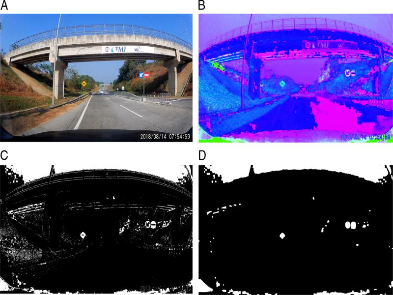
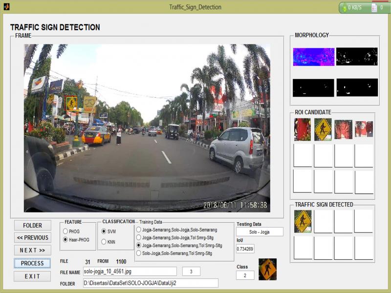
In this research, traffic signs detection is carried out by combining color segmentation in HSI color space and the extraction of Haar–PHOG features. HSI color space can separate traffic signs from complex backgrounds, while Haar–PHOG can emphasize the shape of candidate signs, whether they are circles, diamonds, and squares. In HSI segmentation process, the H and S threshold values are used to obtain red, yellow, and blue sign colors. This is followed by morphology processing to obtain binary images that are free of noise or blob. These two processes result in candidate signs in the form of Region of Interest (ROI).

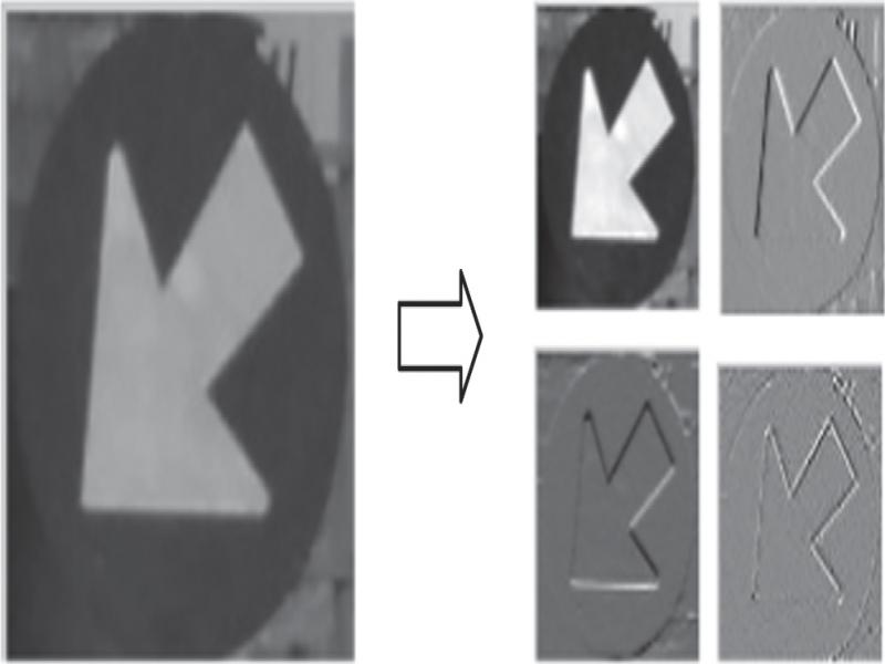
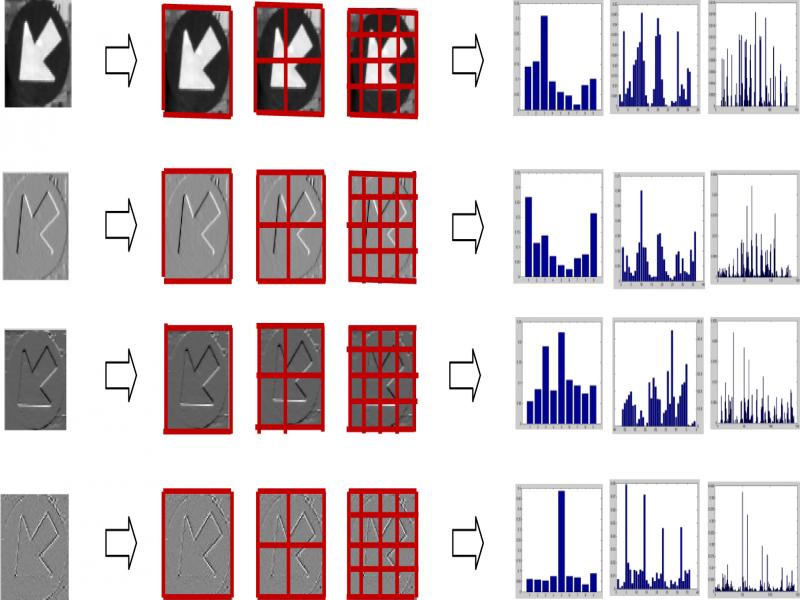
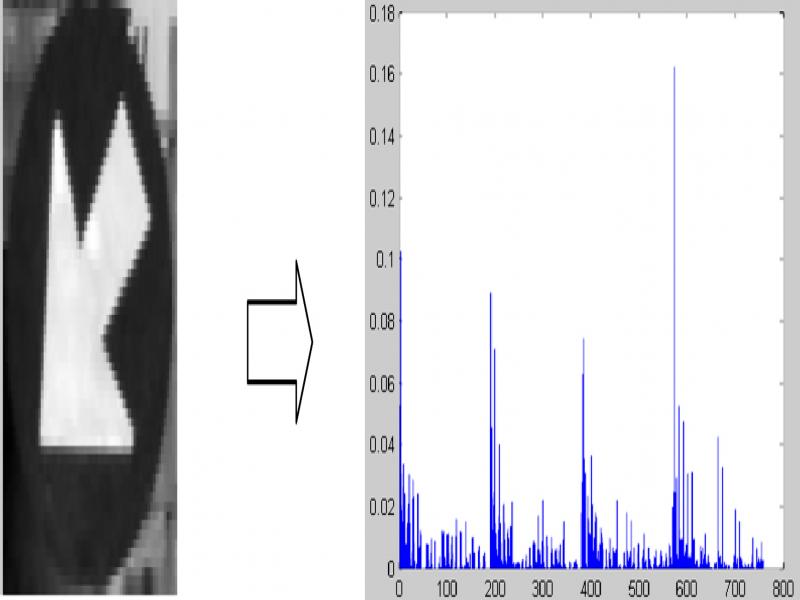
ROI serves as input for the extraction of Haar–PHOG features. Haar–PHOG feature extraction is a combination of Haar and PHOG wavelet transforms. At this stage, ROI is transformed into Haar discrete wavelets to produce four regions of different frequencies of LL, HL, LH, and HH. Each area is extracted for its PHOG features and results in four PHOG feature vectors. This means that the number of features produced in Haar–PHOG feature extraction is four times those of PHOG features. Afterward, each ROI feature candidate is classified using binary SVM to determine whether the ROI is a traffic sign or not.

This research contributes to the extraction of Haar–PHOG features, which emphasize frequency and resolution. Haar–PHOG combines four regions of different frequencies from Haar discrete wavelet transform using PHOG resolution depth level to produce features that are four times those of PHOG.

There are several sections in this paper. The second section describes some previous studies concerning the detection of traffic signs. The third section focuses on describing the proposed method, while the fourth section contains experiments that have been carried out using training data and testing, as well as the application of the proposed feature extraction method. And the fifth section presents conclusions.

Related work

The color and shape of traffic signs are designed uniquely to highlight their presence. To detect traffic signs, some researchers first used color and followed by matching of shape features (Mogelmose et al., 2012). Traffic signs can be captured by a camera as images or video data for transportation monitoring in megacities (Kalistatov, 2019). RGB color segmentation can separate red, yellow, and blue sign colors with the detection accuracy of up to 92% (Ruta et al., 2010). RGB color space normalization was also used to detect red traffic signs by adding an average threshold value and a standard deviation (Zaklouta et al., 2011). In the meantime, Wang (2014) used RGB color segmentation to separate red, blue, and yellow signs from complex backgrounds using an achromatic model with an accuracy of up to 93.2%. In another study, normalized RGB was used to detect traffic signs made up of mostly red and blue using a threshold value based on experimental results. Results show that the use of normalized RGB is better than HSV color space for the detection of red signs. While for the blue sign, HSV is capable of higher detection accuracy compared to normalized RGB (Berkaya et al., 2016).

The use of RGB color space has a drawback against lighting changes that may result in low accuracy. Therefore, there is a need to use a more robust color space, such as HSV (Chen et al., 2013). H and S values are used as input in the Ada boost classification to produce a binary image with the desired color given a value of 1 and vice versa 0. Results of a study using data in bright, cloudy, foggy, and snowy lighting conditions obtained a detection accuracy of 95% (Fleyeh, 2013).

A study on the detection and recognition of speed limits also used the HSV color space. Speed limit sign was detected by training H and S values using the LVQ (Learning Vector Quantization) artificial neural network. This study obtained a speed limit sign detection accuracy of up to 97% (Biswas and Tora, 2014).

Other than HSV, some researchers used HSI to obtain color segmentation that is resistant to lighting changes. Traffic signs of red, yellow, and blue color were detected based on H, S, and I segmentation, while traffic signs of white color were detected based on achromatic color segmentation (Maldonado-Bascon et al., 2007). HSI color space was also used to detect the presence of traffic signs by separating red, yellow, and blue colors using threshold values (Shengchao et al., 2014). In another study, the H color component was used to localize three primary colors (red, blue, and yellow). Yet, another research used morphological and labeling techniques to obtain relevant ROI as candidates for traffic signs (Han et al., 2015).

Another research tried to increase the accuracy of value during the detection process by extracting features after color segmentation. The invariant moment feature is resistant to changes in rotation, scaling, and the translation used to detect fires in tunnels (Dai et al., 2019). Hough transformation was used to determine the features of a circular speed limit sign (Biswas and Tora, 2014). The texture aspect was applied for feature extraction processes such as LBP, which calculates the value pixel intensity at the center point to neighboring pixels that alters binary code obtained back to decimal (Ojala et al., 2002). Another research developed LBP into three DLBP or three-dimensional LBP on different gray-colored images and color images, including RGB, oRGB, YCbCr, YIQ, and HSV color spaces (Banerji et al., 2013a). Meanwhile, the use of LBP for feature extraction in traffic sign images with CSLBP as local features that are combined with global DWT features. Results show that combined features come with higher accuracy compared with separate use of either Discrete Cosine Transform (DCT) or DWT with significantly faster computing speed (He and Dai, 2016).

Research on feature extraction continues to develop, especially with descriptor-oriented features such as HOG. HOG uses bi-directional convolution operations with horizontal and vertical kernels that allow resistance against lighting changes. From the two convolution matrices, edge strength and angle tangent are calculated, and these result in orientation. Each block and cell is calculated for bin orientation of each descriptor, whether it is bin 180° or 360° (Dalal and Triggs, 2005). After successfully detecting pedestrians, HOG feature was used to identify triangular traffic signs (Fleyeh, 2015). HOG divides ROI into intersecting blocks, and each block is further divided into non-intersecting cells. This process was followed by the recognition of traffic signs using SVM multi-class classification, which was then compared with the use of Kd-tree and random forest (Zaklouta and Stanciulescu, 2012). Feature extraction of HOG was also used for traffic signs. Prior to the classification of traffic signs, an ROI of 100  × 100 pixels is obtained, and features are extracted using an eight bin HOG on each cell. The result was then used for the classification process. There are four classifications used: ANN, k-NN, SVM, and Random Forest. Using the GTSDB dataset, it was found that Random Forest classification has a higher level of accuracy compared to other classification methods (Wahyono and Jo, 2014).

HOG feature extraction was developed into HOG-ring(Soetedjo and Somawirata, 2017) and soft HOG or SHOG using symmetry patterns to determine the number of cells in a block. Thus, the number of cells in each block is not the same. GTSDB dataset was used to test SHOG performance compared to HOG, which implemented with genetic algorithms. Results show that SHOG is more promising compared to HOG (Kassani et al., 2016). The performance of HOG feature extraction on traffic signs was also tested with HSI-HOG, which involved HSI color space, and H, S, and I values are extracted using HOG. The three datasets used (GTSRB, GTSDB, and STS/Swedish Traffic Sign) show that HSI-HOG is better than HOG for all datasets (Ellahyani et al., 2016).

In another study, HOG feature extraction was developed into Haar–HOG. In this method, a discrete wavelet transformation with Haar was performed on an ROI image before HOG processing. The ROI was taken from the segmentation process using several different color spaces such as RGB, Grayscale, HSV, and YCbCr. HOG processing on four quadrants of LL, HL, LH, and HH frequencies was then performed. Both features were then tested using SVM on the Caltech, MIT, and UIUC datasets. Results show that Haar–HOG characteristics had better performance compared to those of HOG (Banerji et al., 2013b).

The characteristics of an object can also be seen as a pyramid consisting of several levels. Similarly, PHOG feature extraction views an image as an HOG pyramid (Adnan et al., 2015). PHOG uses Canny edge detection by calculating edge strength and direction gradients. PHOG feature vector is calculated based on the sum of feature vectors from each level (Bosch and Zisserman, 2007).

Research related to the detection of traffic signs using PHOG feature extraction performed segmentation stages by converting RGB to Gaussian color models and screening the area or extent of the candidate ROI. The results of this stage were then followed by feature extraction using PHOG. However, the use of Canny edge detection has a drawback in the form of noise coming from complex environments or backgrounds. Traffic signs used in this study had ether circle, triangle, inverted triangles, or diamond shapes. Results show that the use of PHOG* feature extraction followed by a binary SVM detection had a better performance compared to PHOG (Li et al., 2015). The detection process can be made even faster using Compute Unified Device Architecture (CUDA) (Razian and Mahvash Mohammadi, 2017) or with the help of tracing using Kalman filtering method (Espejel-García et al., 2017).

Proposed method

Traffic sign detection is important as it serves as input for the next stage of traffic sign recognition. This research used a combination of color segmentation and feature extraction of traffic signs to improve detection performance. The initial stage started with color segmentation using HSI and morphology to produce a binary image that contains ROI as a traffic sign candidate. In the next step, Haar–PHOG feature extraction was used to get the form of traffic signs. This feature extraction emphasizes highlighting contour edges with Haar wavelet transforms that produced four times the number of features compared to PHOG features. In the final stage, SVM classification was used to determine if the ROI feature was a traffic sign or not. The stages of the proposed method are depicted in Figure 1.

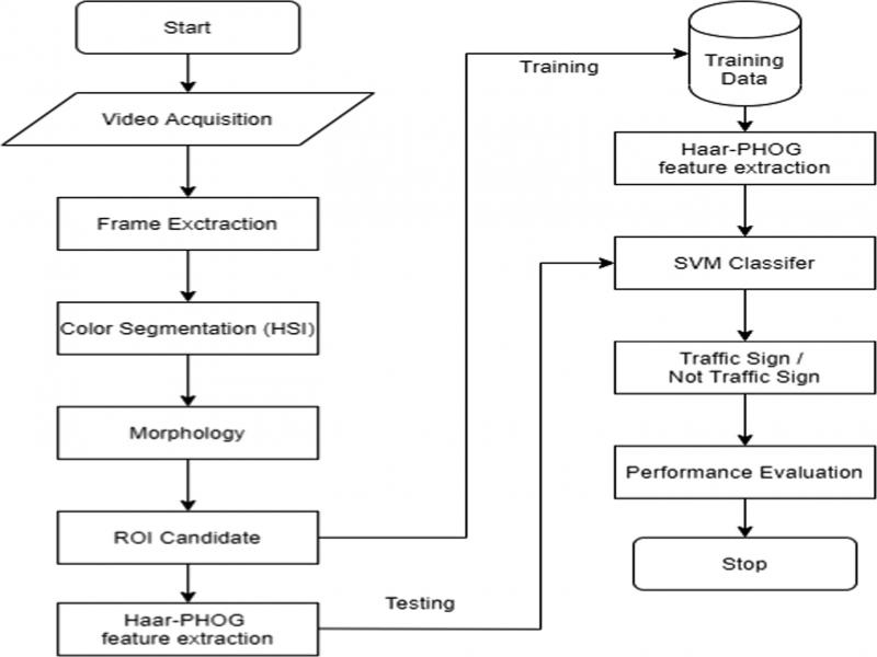
Figure 1:

Color segmentation of traffic sign

Segmentation is aimed at separating images of traffic signs from complex backgrounds. Traffic signs generally come in unique colors that segmentation based on color is an option. RGB color space can be an option because it requires low computational level. However, RGB color space is very vulnerable to changes in light intensity that may result in lower accuracy. In this study, HSI color space was used because it is based on human color perception and is relatively more stable to changes in light. The range of H and S values used to obtain basic colors of traffic signs is shown in Table 1 (Shengchao et al., 2014).

Table 1.

Range of hue and saturation threshold values.

The results of the segmentation process are binary images, where white is the object, while black is the background. The segmentation process still leaves blobs that are very annoying noise and may cause longer search time (Fig. 2C). Therefore, a morphological process is needed in the form of an opening operation, which is an erosion operation followed by a dilatation operation to reduce the blob and leave the candidate as ROI of the traffic sign (Fig. 2D).

Figure 2:

Haar–PHOG feature extraction

Haar wavelet transform

Wavelet function is a mathematical function of certain properties, including oscillating around zero, such as sine and cosine functions, and is localized in the time domain, which means that when the domain value is relatively large, the wavelet function is worth zero. Wavelets are divided into two types of father wavelet (ϕ) and mother wavelet (ψ), with the following characteristics (Daubechies, 1992):

(1)

${\int }_{-\infty }^{\infty }\phi (x)dx=1,$

(1)

(2)

${\int }_{-\infty }^{\infty }\psi (x)dx=0.$

Haar wavelet is a set of two-dimensional Haar functions that can be used to encode local appearance of an object. Haar function is defined as follows (Daubechies, 1992):

(3)

$\varphi (x)=\{\begin{array}{c}1,0⩽x<\frac{1}{2}\\ -1,\frac{1}{2}⩽x<1\\ 0,\mathrm{others}\end{array}.$

Haar wavelet transform decomposes a discrete signal into two sub-signals, each of which is half the original size. One sub-signal represents the average or trend, while the other sub-signal is the difference or fluctuation. A signal f = (f₁ , f₂ , f₃, …, f_N), where N is a positive integer will produce sub-signals as trend a_m  = (a₁, a₂, a₃, …, a_N/2), which is obtained from the following equation (Arora et al., 2014):

(4)

$a_m=\frac{f_{2m-1}+f_{2m}}{\sqrt{2}}.$

Meanwhile, the sub-signal that states fluctuation is denoted as d_m = (d₁, d₂, d₃, …, d_N/2) and is formulated in the following equation (Arora et al., 2014):

(5)

$d_m=\frac{f_{2m-1}-f_{2m}}{\sqrt{2}}.$

PHOG feature extraction

PHOG feature extraction is a development of the HOG feature and has been used extensively in object detection, classification, and recognition of facial expressions, as well as vehicle classification. PHOG divides ROI into several regions depending on level depth. At level 0, feature extraction is carried out at full ROI, while at level 1, the process is carried out by dividing ROI into four equal parts, and at level 2, the ROI is divided into 16 parts, and so on. The resulting features are the sum of features at the current level plus all features from the previous level. At level 2, the resulting features are a combination of features from level 0, level 1, and level 2. Stages in determining PHOG features include (Bosch and Zisserman, 2007):

1. Candidates for traffic signs in the form of ROI are subject to edge detection operations using Canny detectors to obtain edge contours.

2. ROI is broken down into cells at the pyramid level or its hierarchy, where the number of cells is determined c_j = 2^j.

3. At each level of the pyramid, HOG feature is calculated to get a histogram that represents local form features.

4. PHOG features are the total number of HOG feature vectors from each pyramid level.

In this study, PHOG feature extraction was calculated at level 2 depth, so that a total PHOG feature vector obtained is (1 × 9) + (4 × 9) +(16 × 9) = 189. This feature vector was used as training data in the next stage.

Extraction of Haar–PHOG feature

Haar–PHOG feature extraction is a combination of Haar wavelet transformation with PHOG feature extraction, where the Haar wavelet transformation process is performed before PHOG. In this study, level 1 Haar wavelet transform was used. The extraction of Haar–PHOG feature started with taking candidate ROI, followed by Haar wavelet transformation that four regions with different frequencies were obtained (Fig. 3). Each of these regions then underwent PHOG process at level 2 depth (Fig. 4). The final result of this feature extraction is a combination of features from the four transformed regions (Fig. 5). The number of features generated from Haar–PHOG is four times those of PHOG.

Figure 3:

Figure 4:

Figure 5:

Support vector machine (SVM)

Classification is used to categorize an entity into a specific group. As a classifier, SVM plays an essential role in determining ROI selected from a range of images to determine if it is a traffic sign or not (Wahyono and Jo, 2014). In this study, binary SVM was used to classify an entity into a group of traffic signs (+1) or non-traffic signs (−1). SVM classification was used to find the optimal solution $f:X\to \{+1,-1\}$ with n sample of data pairs $\{(x_i,y_i)\}$ where $x_i\in X$ ROI feature data is and $y_i\in \{+1,-1\}$ is the label. SVM separates two classes of sign and non-sign data using hyperplane {w, b} which satisfies x.w^T + b = 0,  with hyperplane H₁:x_i.w^T + b = 1 and H₂:x_i.w^T + b = −1 with the distance between hyperplanes is $\frac{2}{\parallel w\parallel }$ (Dalal and Triggs, 2005). The data used for implementation are HOG, PHOG, and Haar–PHOG features from ROI of traffic signs as positive training data with +1 label and non-traffic signs as negative data with label −1. Meanwhile, the data used for testing are several candidates for traffic signs in the form of ROI obtained from a frame of images that is counted for its features and then used as input for SVM classification to determine whether the ROI is a traffic sign or otherwise.

Experiment

Data

The data used in this research were taken from three roads of Semarang – Solo, Solo – Yogyakarta, Semarang – Yogyakarta, and the Semarang – Salatiga toll road. Data (images) were taken using a Xiaomi Yi dashcam of 1,080 × 1,920 pixel resolution, a capture angle of up to 160°, and a speed of 30 frames per second. The vehicle was on normal speed on the three public roads, depending on traffic condition, and was adjusted to the speed limit of 60 km/h and a maximum of 80 km/h, while cruising down the Semarang – Salatiga toll road. This experiment used three roads to test one road. In the first training, the Semarang-Solo, Solo-Yogyakarta, and Semarang-Yogyakarta road sections were used as training, while the Semarang-Salatiga toll road was used for testing. In the second training, data from Solo-Yogyakarta, Semarang-Yogyakarta, and the Semarang-Salatiga toll road for training, whereas the Semarang-Solo road was used as testing, and so on. The training data used were ROI of traffic signs as positive data and ROI of non-traffic signs as negative data (Figs. 6A, 7), while the data used as test data were image frames extracted from video data on each road section (Fig. 6B). The experiments use Matlab on a computer with Core(TM) i5-4200M CPU @2.50 GHz. The composition of training and testing data are given in Table 2.

Table 2.

Composition of training and testing data.

Color	Hue	Saturation
Red	H ≥ 290 or H ≤ 15	S ≥ 10
Yellow	20 ≤ H ≤ 65	S ≥ 150
Green	180 < H ≤ 280	S ≥ 10

Figure 6:

Figure 7:

Result

Experiments were carried out by using training data and test data on four roads. Taking four regions, including low-frequency LL, medium frequency (HL and LH), and high-frequency HH areas obtained from level 1 Haar wavelet transform and level 2 PHOG feature extraction, results in data as shown in Tables 3–11.

Table 3.

Confusion matrix of Solo-Yogyakarta road.

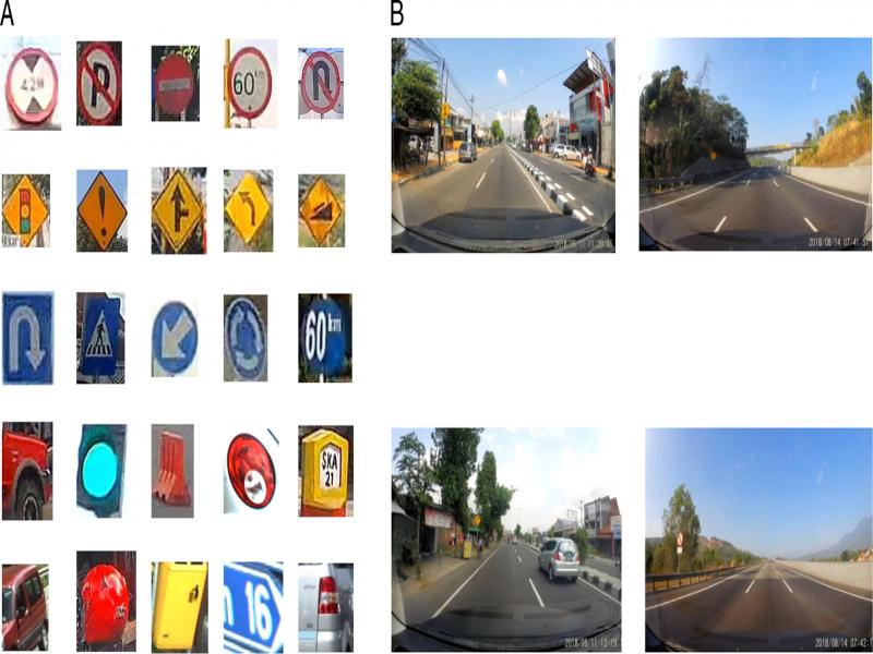
	Training data (ROI)
Road	Positive	Negative	Testing data (frame)	Number of traffic sign
Solo-Yogyakarta	1,500	1,500	1,100	1,153
Semarang-Yogyakarta	1,500	1,500	950	929
Semarang-Solo	1,500	1,500	1,000	1,099
Semarang – Salatiga Toll Roads	1,500	1,500	950	982

Table 4.

Confusion matrix of Semarang-Yogyakarta road.

					Haar–PHOG
	HOG		PHOG		LL		LL HL LH		LL HL LH HH
Solo-Yogyakarta	Predict (No)	Predict (Yes)	Predict (No)	Predict (Yes)	Predict (No)	Predict (Yes)	Predict (No)	Predict (Yes)	Predict (No)	Predict (Yes)
Actual (No)	2,328	109	2,213	112	2,317	56	2,308	38	2,304	41
Actual (Yes)	32	1,044	147	1,041	43	1,097	52	1,115	56	1,112

Table 5.

Confusion matrix of Semarang-Solo road.

					Haar–PHOG
	HOG		PHOG		LL		LL HL LH		LL HL LH HH
Semarang-Yogyakarta	Predict (No)	Predict (Yes)	Predict (No)	Predict (Yes)	Predict (No)	Predict (Yes)	Predict (No)	Predict (Yes)	Predict (No)	Predict (Yes)
Actual (No)	2,492	132	2,356	144	2,471	84	2,451	56	2,451	52
Actual (Yes)	59	797	195	785	80	845	100	873	100	877

Table 6.

Confusion matrix of Semarang-Salatiga toll road.

					Haar–PHOG
	HOG		PHOG		LL		LL HL LH		LL HL LH HH
Semarang-Solo	Predict (No)	Predict (Yes)	Predict (No)	Predict (Yes)	Predict (No)	Predict (Yes)	Predict (No)	Predict (Yes)	Predict (No)	Predict (Yes)
Actual (No)	1,896	232	1,807	172	1,881	161	1,865	145	1,868	145
Actual (Yes)	27	867	116	927	42	938	58	954	55	954

Table 7.

Comparison of accuracy HOG, PHOG, and Haar–PHOG features.

					Haar–PHOG
	HOG		PHOG		LL		LL HL LH		LL HL LH HH
Semarang-Salatiga toll	Predict (No)	Predict (Yes)	Predict (No)	Predict (Yes)	Predict (No)	Predict (Yes)	Predict (No)	Predict (Yes)	Predict (No)	Predict (Yes)
Actual (No)	1,504	123	1,421	162	1,427	103	1,433	79	1,431	73
Actual (Yes)	13	859	96	820	90	879	84	903	86	909

Table 8.

Comparison of precision HOG, PHOG, and Haar–PHOG features.

	Accuracy (%)
	HOG	PHOG	Haar–PHOG
Road	Fleyeh (2015)		LL	LL HL LH	LL HL LH HH
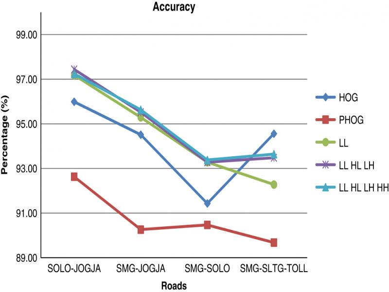
Solo-Yogyakarta	95.99	92.63	97.18	97.44	97.24
SMG-Yogyakarta	94.51	90.26	95.29	95.52	95.63
SMG-Solo	91.43	90.47	93.28	93.28	93.38
SMG-SLTG-Toll	94.56	89.68	92.28	93.48	93.64

Table 9.

Comparison of recall HOG, PHOG, and Haar–PHOG features.

	Precision (%)
	HOG	PHOG	Haar–PHOG
Road	Fleyeh (2015)		LL	LL HL LH	LL HL LH HH
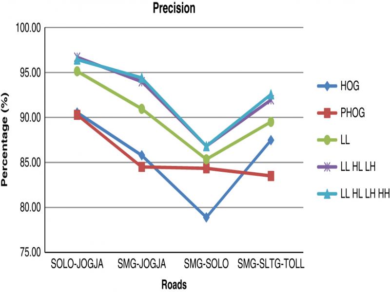
Solo-Yogyakarta	90.55	90.29	95.14	96.70	96.44
SMG-Yogyakarta	85.79	84.50	90.96	93.97	94.40
SMG-Solo	78.89	84.35	85.35	86.81	86.81
SMG-SLTG-Toll	87.47	83.50	89.51	91.96	92.57

Table 10.

The training time of HOG, PHOG, and Haar–PHOG features.

	Recall (%)
	HOG	PHOG	Haar–PHOG
Road	Fleyeh (2015)		LL	LL HL LH	LL HL LH HH
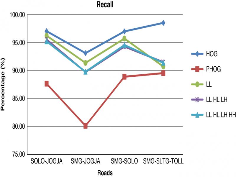
Solo-Yogyakarta	97.03	87.63	96.23	95.54	95.21
SMG-Yogyakarta	93.11	80.10	91.35	89.72	89.76
SMG-Solo	96.98	88.88	95.71	94.27	94.55
SMG-SLTG-Toll	98.51	89.52	90.71	91.49	91.36

Table 11.

Testing time of HOG, PHOG, and Haar–PHOG features.

	Training time (sec)
			Haar–PHOG
Road	HOG	PHOG	LL	LL HL LH	LL HL LH HH
Solo-Yogyakarta	148.38	512.66	15.73	27.31	32.78
SMG-Yogyakarta	148.02	555.50	16.25	27.05	32.59
SMG-Solo	168.98	537.25	15.73	28.73	33.66
SMG-SLTG-Toll	165.03	583.41	18.06	32.05	35.61
Average	157.60	547.20	16.45	28.79	33.66

Graphs showing simple comparisons of accuracy, precision, and recall are depicted in Figures 8–10.

Figure 8:

Figure 9:

Figure 10:

HOG feature uses 16 × 16 blocks and 8 × 8 cells. Traffic sign ROIs have 128 × 128 pixels and resulted in intersecting blocks of 15 × 15 or 225 blocks. If each block is divided into four cells, then each cell will generate nine features, that there is a total of 225 × 4 × 9 or 8,100 features. For PHOG feature of the same ROI dimension (128 × 128) and at level 2 pyramid, a total feature of 9 + 36 + 144 or 189 is obtained. Meanwhile, for Haar–PHOG feature of 128 × 128 ROI dimension, and at level 2 pyramid, as well as level 1 wavelet transform, a feature of 189 is obtained at a low-frequency wavelet coefficient (LL). For low and mid-frequency wavelet coefficient (LL, HL, and LH), the features obtained are 189 × 3 or 567. And if all features from all frequencies, including that of high frequency (HH) are calculated, a feature of 189 × 4 or 756 is obtained. Tables 7 to 11 show that the use of HOG feature results in better performance compared to PHOG. This is only reasonable as there are more features used, 8,100 compared to 189. However, when it comes to training speed, PHOG is way much slower than HOG. On another front, comparison for the use of HOG and Haar–PHOG features shows better performance by the latter, despite the fact that it uses much fewer features compared to HOG, with only 189, 567, or 756, depending on the frequency used, compared to the burgeoning 8,100. And just as with PHOG, training speed for Haar–PHOG is also much faster compared to that of HOG. When we compare the advantages of both PHOG and Haar–PHOG for level 2 pyramid for standard ROI of 128 × 128, as shown in Tables 7–9, it is clear that Haar–PHOG contributes significantly to improved performance, in terms of accuracy, precision, and recall. This also applies to all frequencies of LL, HL, and LH, as well as LL, HL, LH, and HH. Even though PHOG has fewer features compared to Haar–PHOG, however the training time for Haar-PHOG is significantly less than those of PHOG.

What is more interesting is the contribution that Haar–PHOG feature has on traffic sign detection for wavelet coefficients of LL, HL, LH, and HH. Even though the number of features for LL wavelet is only 189, the average addition of HL, LH, and HH wavelet with an increasing number of features of 567 and 756 does not significantly affect performance. This is evident in a relatively stable accuracy of 94%, with an average increase in accuracy of 2%, from 90.24 to 92.56%, which is balanced with an average 1% decrease in recall from 93.50 to 92.72%.

Conclusion

Results from this experiment show that the use of Haar–PHOG feature extraction followed by SVM classification generally results in better accuracy, precision, and recall values compared to HOG and PHOG feature extraction. Extraction of Haar–PHOG features can produce up to four times the number of features compared to those of PHOG, depending on the selection of wavelet coefficient regions. The Haar–PHOG feature proposed has a better performance compared to that of HOG and PHOG in terms of detection capability, training time, and testing time. Haar–PHOG is superior in almost all criteria. These include relatively small features yet better accuracy and precision, compared to HOG and PHOG. In terms of training time, Haar–PHOG is five times faster than HOG and is 20 times faster than PHOG (see Table 10). For a testing time, Haar–PHOG is also five times faster than HOG and is comparable to PHOG (see Table 11).

The road with the highest accuracy, precision, and recall values compared to the other three is the Solo-Yogyakarta road segment. The extraction of the Haar–PHOG feature can contribute to differentiating the sign and non-sign classes. This relatively small FN or FP values result in greater recall and precision values. Meanwhile, the results of the accuracy, recall, and precision values for the Semarang-Salatiga toll road are not too high, despite the fact that the background of the traffic signs is not too complex, and that traffic signs can clearly be seen. One possibility is relatively stable, and the fast vehicle speed of between 60 and 80 km/hr. This is in stark contrast to the other roads where the vehicle had to run relatively slower, depending on traffic conditions. There are still plenty of possibilities for the use of Haar–PHOG feature in further researches, especially with the use of different wavelet and transformation levels. The PHOG feature can also be extended for a more effective pyramid level of choice. This is because a higher level of choice results in a greater dimension of resulting features. Nonetheless, its significance in performance still requires further studies. Furthermore, the data taken from four roads in this research are still limited to separately extracted frames of images. This means that real-time data processing can help improve results from this research.

	Testing time (milliseconds)
			Haar–PHOG
Road	HOG	PHOG	LL	LL HL LH	LL HL LH HH
Solo-Yogyakarta	18.40	3.90	3.00	4.50	5.00
SMG-Yogyakarta	19.00	4.40	2.60	4.40	5.00
SMG-Solo	19.50	4.00	2.60	4.40	5.10
SMG-SLTG-TOLL	19.80	4.00	2.80	4.60	5.30
Average	19.18	4.08	2.75	4.48	5.10