
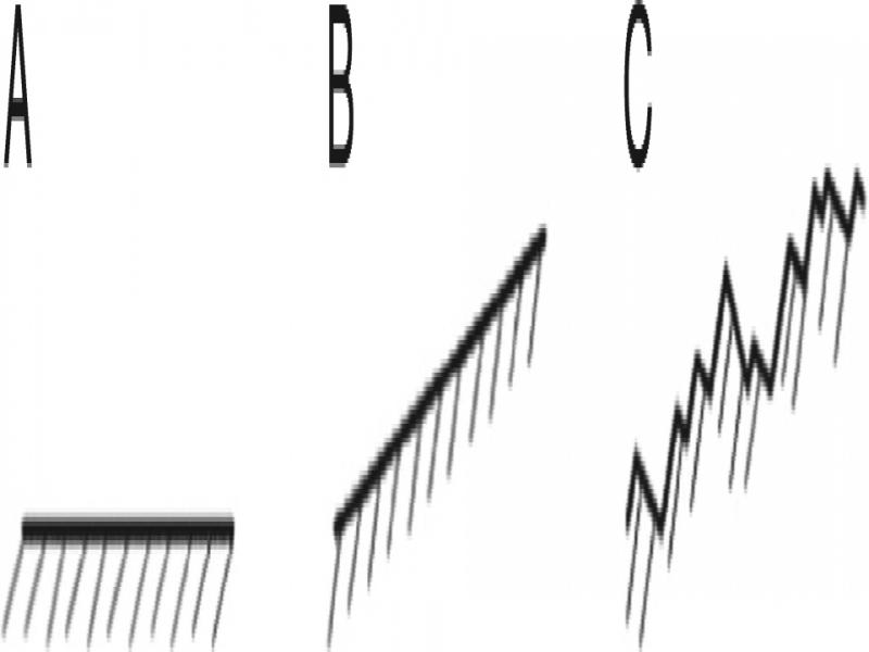
Figure 1:
Examples of surface classes: (A) smooth without slope, (B) smooth with some slope, and (C) with both slope and roughness/texture.
Table 1.
Comparison of 3D surface reconstruction techniques.
| Time of flight | Stereo vision | Optical fiber | Structure light | |
|---|---|---|---|---|
| Working distance | Long | Medium | Short | Short–medium |
| Vision field | Medium | Lenses dependent | Narrow | Medium |
| Cost | High | Medium | Medium | Low |
| Power | Low | Low | Low | Low |
| Accuracy | Medium | Medium | High | Medium |
| Speed | Fast | Fast | Slow | Medium |
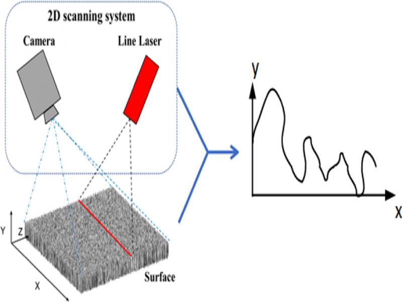
Figure 2:
The principle of data acquisition; working with laser-projected images (left side) to extract a surface profile along x-axis (right side).
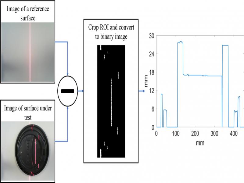
Figure 3:
Basic image processing workflow for the proposed system; difference between test and reference images plus binarization (left side), where the extracted laser provides the surface 1D profile.
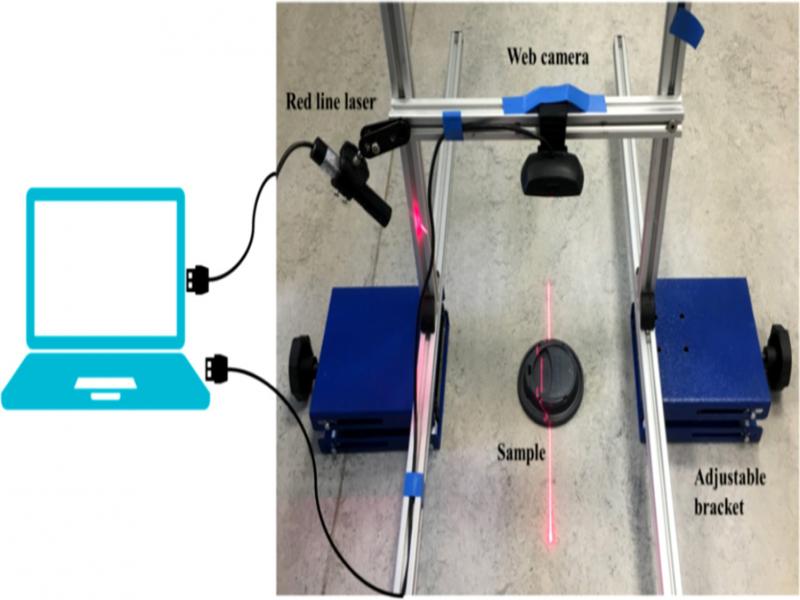
Figure 4:
The experimental setup of our surface level measurement system.
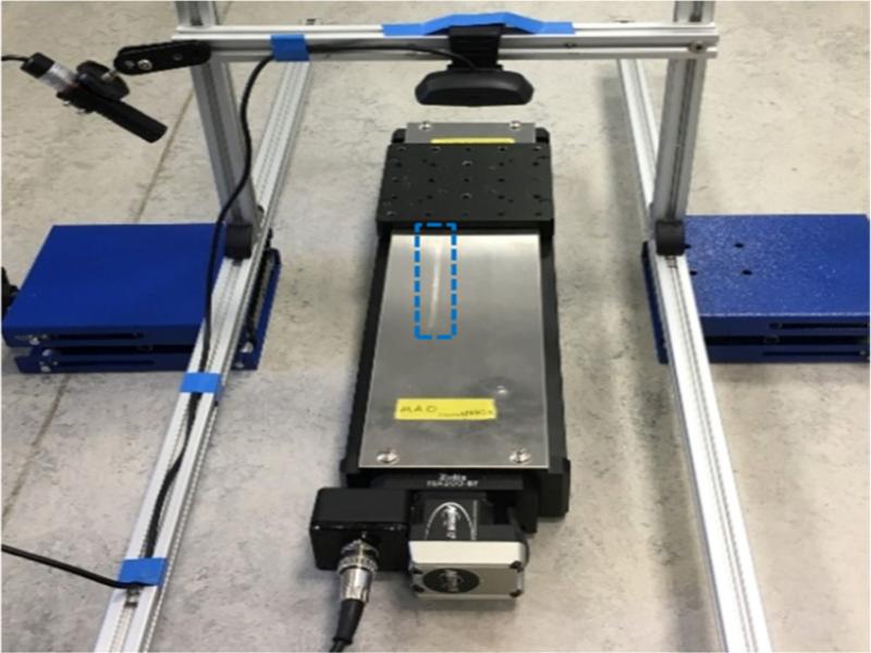
Figure 5:
2D scanning system with a linear actuator; 2D map is obtained from attaching 1D profiles, where the laser line is highlighted in a dashed rectangle.
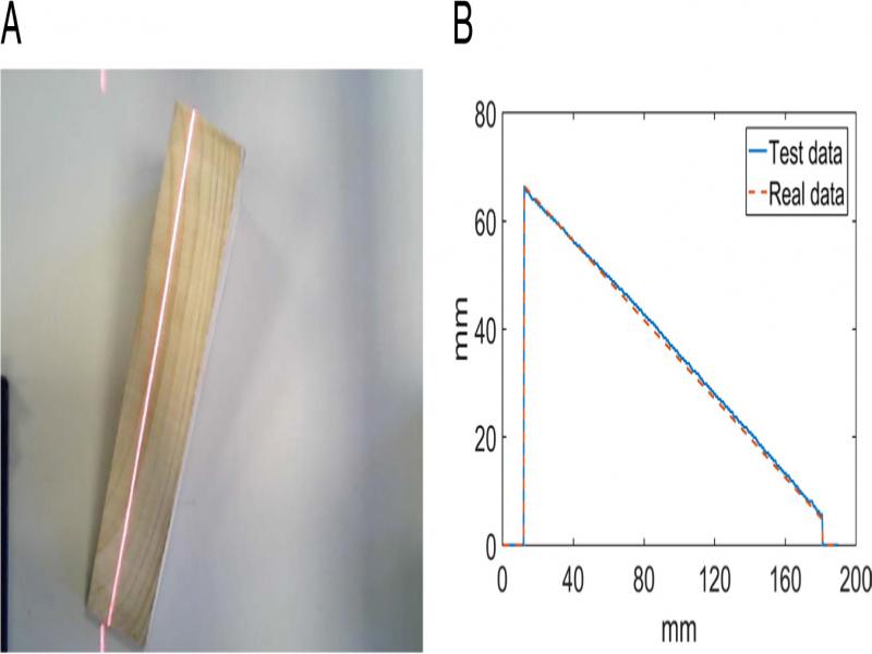
Figure 6:
The experimental results for a simple surface (woody wedge), including (A) test image with projected laser line, and (B) obtained levelness H(x) from the wedge sample.
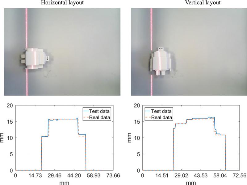
Figure 7:
The experimental results for a complex surface (robot toy), including test image with projected laser line (first row), and obtained levelness H(x) from the sample (second row). Working distance is 25 cm, and the sample is placed horizontally and vertically.
Table 2.
Evaluated cases for complex surface measurement with horizontal layout.
| Horizontal layout | |||
|---|---|---|---|
| Dist. | Images | 1D Profile H(x) | MSE |
| 19 cm | 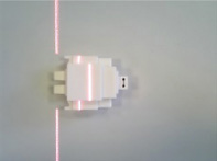 | 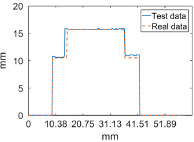 | 0.427 |
| 22 cm | 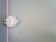 | 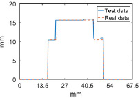 | 0.457 |
| 25 cm | 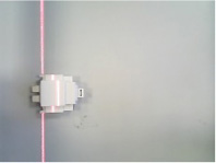 | 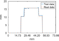 | 0.366 |
| 28 cm | 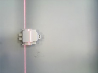 | 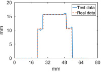 | 0.375 |
| 31 cm | 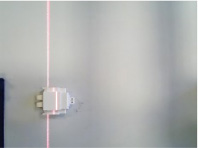 | 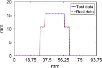 | 0.014 |
| Mean square error (MSE) | 0.328 | ||
Table 3.
Evaluated cases for complex surface measurement with vertical layout.
| Vertical layout | |||
|---|---|---|---|
| Dist. | Images | 1D Profile H(x) | MSE |
| 19 cm | 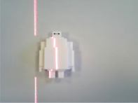 | 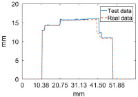 | 0.366 |
| 22 cm | 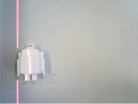 | 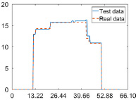 | 0.209 |
| 25 cm | 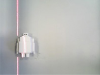 | 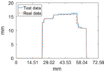 | 0.220 |
| 28 cm | 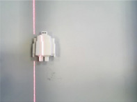 | 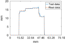 | 0.073 |
| 31 cm | 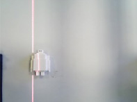 | 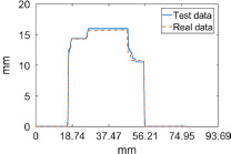 | 0.161 |
| Mean square error (MSE) | 0.206 | ||
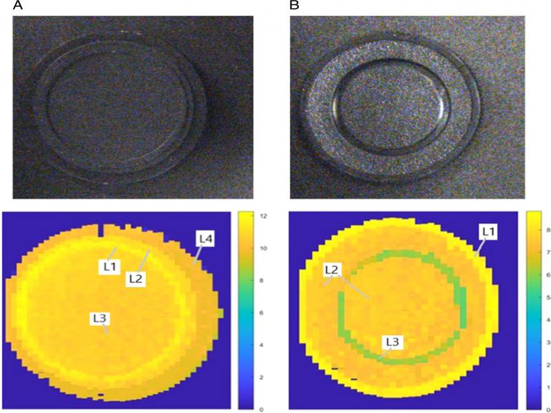
Figure 8:
Real image (top) and obtained 2D levelness maps (bottom) from the surface of two samples (cap A and cap B). The levelness H(x,y) is measured by the color bar in mm.