
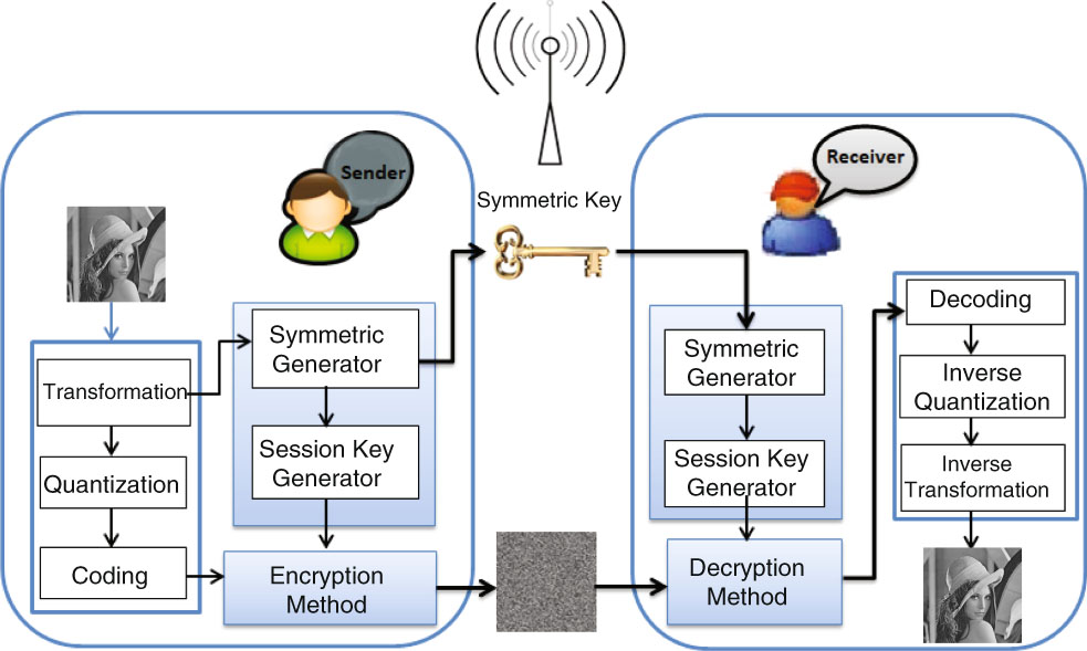
Figure 1
The proposed compression–encryption model.
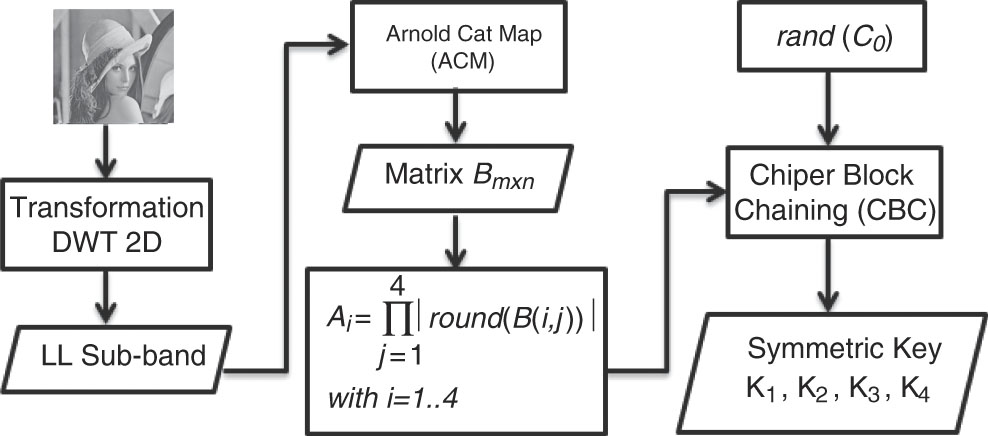
Figure 2
Symmetric Key Generation Algorithm.
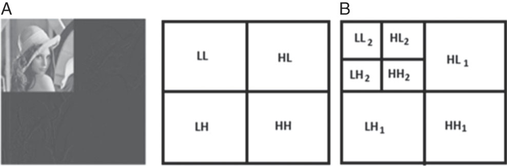
Figure 3
DWT decomposition 2D (a) one level (b) two levels.
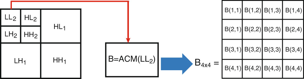
Figure 4
Formation of matrix B from the result of LL sub-band element scrambling using ACM method.
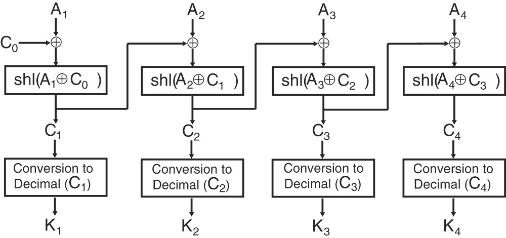
Figure 5
Formation of symmetric keys K1, K2, K3, and K4.
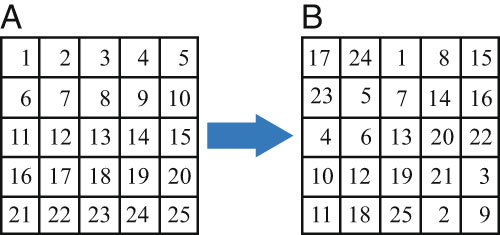
Figure 6
(a) Initial cipher block of size 5×5, (b) session key KG3 which is formed using the proposed algorithm.
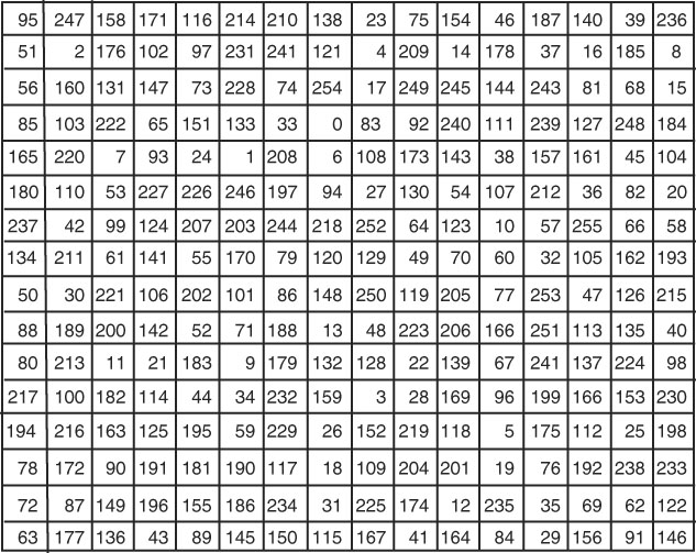
Figure 7
Example of key session KG4 which is randomly generated from the value of symmetric key K4 using the proposed algorithm.
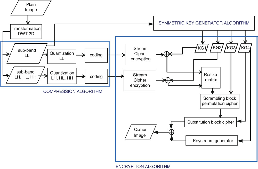
Figure 8
Detailed proposed image compression–encryption model on the sender side.

Figure 9
Illustration of quantization result in binary form The bits are then grouped into 8 bit sized blocks, which produces 71 179 1 (in decimal), as shown in Figure 10.

Figure 10
Illustrated by data coding results.
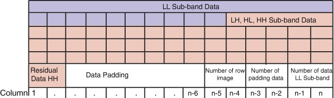
Figure 11
The process of resizing the encrypted LL, LH, HL, and HH sub-bands data from the column vector to a matrix of size m × n 4) Divide the matrix produced in Step 4 into b × k blocks to do the process of block permutation cipher using session key KG3. The goal is to randomize the element.
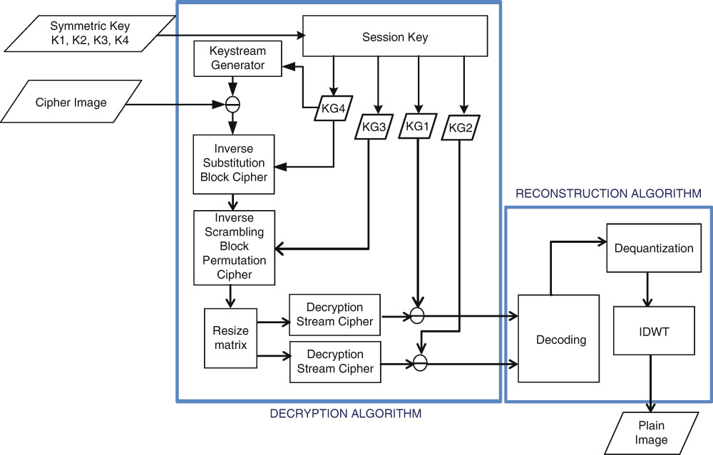
Figure 12
Detailed propoed image decryption–reconstruction model on the receiver side.
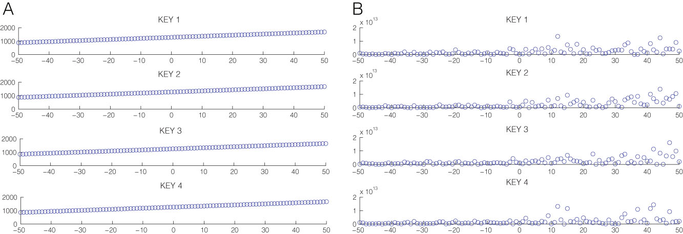
Figure 13
Symmetric key values of Lena images with different intensities. (a) Without using the proposed algorithm and (b) using the proposed algorithm.
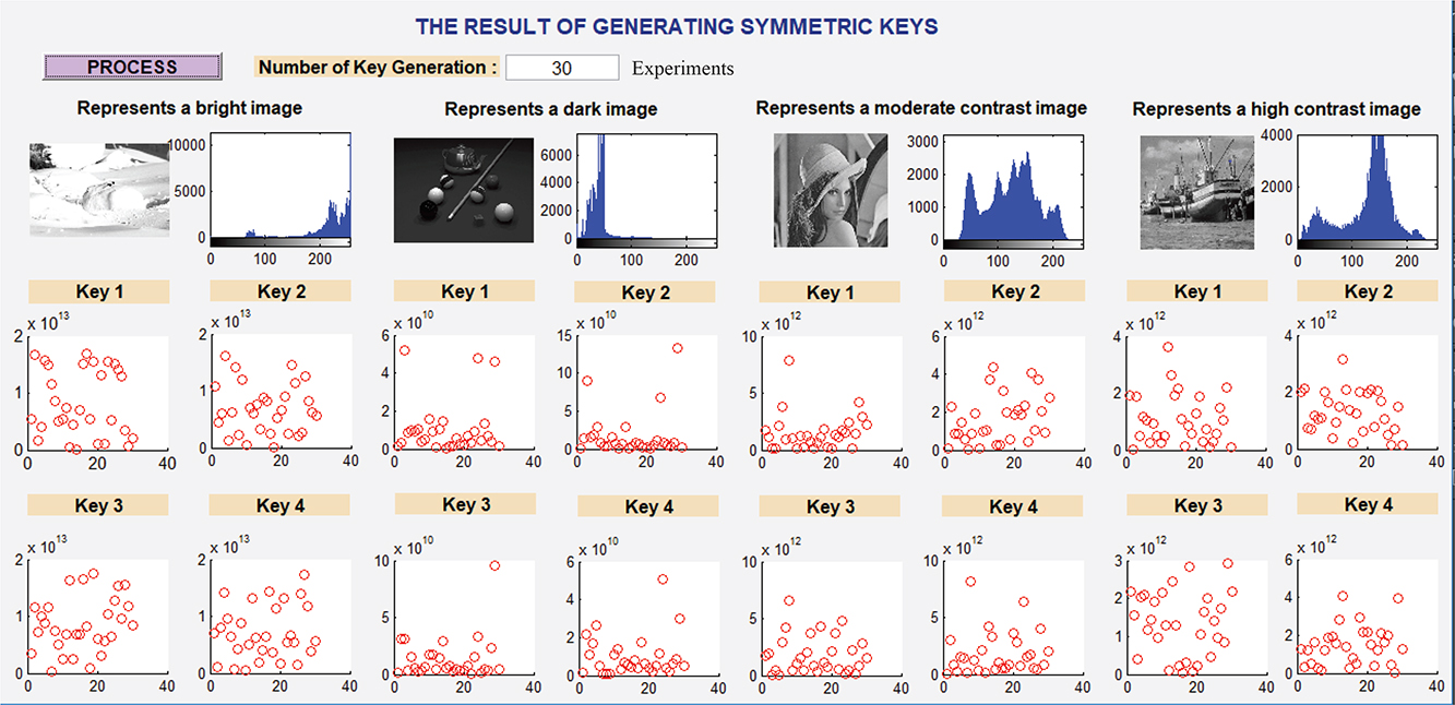
Figure 14
Symmetric keys generated in 30 experiments using Artichare, Pool, Lena, and Boat images.
Table 1
Result of Run-Test test to evaluate the randomness of the symmetric keys.
| Test Image Data | Symmetric Key | P-Value | Conclusion | Test Image Data | Symmetric Key | P-Value | Conclusion |
|---|---|---|---|---|---|---|---|
| Artichare | K1 | 0.930 | Random | Lena | K1 | 0.168 | Random |
| K2 | 0.154 | Random | K2 | 1.000 | Random | ||
| K3 | 0.930 | Random | K3 | 0.670 | Random | ||
| K4 | 1.000 | Random | K4 | 0.624 | Random | ||
| Pool | K1 | 0.145 | Random | Boat | K1 | 0.727 | Random |
| K2 | 1.000 | Random | K2 | 0.593 | Random | ||
| K3 | 0.565 | Random | K3 | 0.353 | Random | ||
| K4 | 0.234 | Random | K4 | 0.098 | Random |
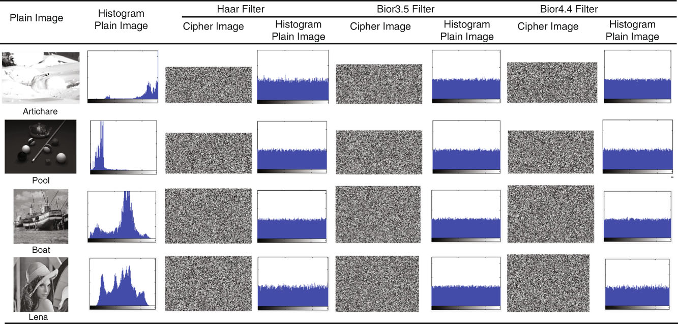
Figure 15
Result of visual analysis to cipher image.
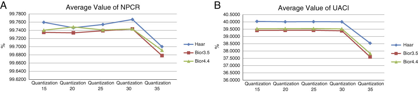
Figure 16
Average value of (a) NPCR, (b) UACI using the four testing images.
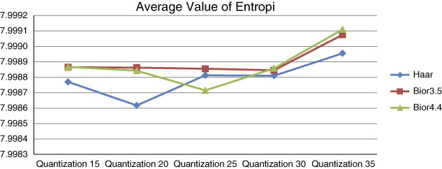
Figure 17
The average value of entropy from four testing images.
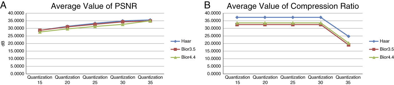
Figure 18
Average value of (a) PSNR, (b) compression ratio of the four testing images.
Table 2
The average of PSNR, UACI, entropy, CR, PSNR values and encryption and decryption process times using 30 different keys.
| File | Classification | NPCR | UACI | Entropy | CR | PSNR | Tencryption (seconds) | Tdecryption (seconds) |
|---|---|---|---|---|---|---|---|---|
| Artichare | Bright image | 99.7554 | 59.9266 | 7.9988 | 37.2500 | 36.0186 | 12.8361 | 18.1816 |
| Pool | Dark image | 99.7546 | 30.7441 | 7.9985 | 37.0757 | 36.4626 | 11.2455 | 14.7797 |
| Lena | Moderate contrast image | 99.7535 | 34.7743 | 7.9989 | 37.3047 | 35.7978 | 14.8640 | 19.8693 |
| Boat | High contrast image | 99.7548 | 34.6731 | 7.9989 | 37.3047 | 34.3238 | 14.9430 | 19.8642 |
Table 3
Comparison of NPCR and UACI values between the proposed method and the method in Belazi et al. (2017), Hamdi et al. (2017), and Zhang and Tong (2017).
| NPCR | UACI | |||||||||
|---|---|---|---|---|---|---|---|---|---|---|
| Citra | Size | Classification | Proposed | Ref (Hamdi et al., 2017) | Ref (Belazi et al., 2017) | Ref (Zhang and Tong, 2017) | Proposed | Ref (Hamdi et al., 2017) | Ref (Belazi et al., 2017) | Ref (Zhang and Tong, 2017) |
| peppers | 512×512 | High contrast | 99.7391 | 99.9676 | - | 99.6100 | 34.3270 | 33.3208 | - | 33.4700 |
| Lena | 512×512 | Moderate contrast | 99.7482 | 99.9150 | - | 99.5900 | 34.7650 | 33.5107 | - | 33.4200 |
| barbara | 512×512 | Moderate contrast | 99.7604 | 99.3656 | - | 99.5700 | 32.6374 | 33.4989 | - | 33.2900 |
| Average | 99.7492 | 99.7494 | - | 99.5900 | 33.9098 | 33.4435 | - | 33.3933 | ||
| Lena | 256×256 | Moderate contrast | 99.7360 | 99.8817 | 99.5895 | - | 34.7258 | 33.6860 | 33.4646 | - |
| house | 256×256 | Moderate contrast | 99.7742 | 98.9948 | 99.6353 | - | 35.5474 | 33.9622 | 33.4534 | - |
| airplane | 256×256 | Bright image | 99.7833 | 99.6680 | 99.5989 | - | 46.2548 | 33.2705 | 33.4396 | - |
| Average | 99.7645 | 99.5148 | 99.6079 | - | 38.8427 | 33.6396 | 33.4525 | - | ||
Table 4
Comparison of entropy value between our proposed model with Belazi et al. (2017) and Zhang and Tong (2017).
| Entropy | |||||
|---|---|---|---|---|---|
| Citra | Size | Classification | Proposed | Ref (Belazi et al., 2017) | Ref (Zhang and Tong, 2017) |
| Airplane | 512×512 | Bright image | 7.9988 | 7.9024 | 7.9931 |
| house | 512×512 | Moderate contrast | 7.9990 | 7.9027 | 7.9931 |
| Lena | 512×512 | Moderate contrast | 7.9989 | 7.9030 | 7.9929 |
| barbara | 512×512 | Moderate contrast | 7.9989 | 7.9025 | 7.9917 |
| Average | 7.9989 | 7.90265 | 7.9927 | ||
Table 5
Comparison of PSNR and CR values between images produced using the proposed and image produced by Hamdi et al. (2017), and Kumar and Vaish (2017).
| PSNR | CR | ||||||
|---|---|---|---|---|---|---|---|
| Citra | Size | Classification | Proposed | Ref (Hamdi et al., 2017) | Ref (Kumar and Vaish, 2017) | Proposed | Ref (Kumar and Vaish, 2017) |
| peppers | 512×512 | High contrast | 34.3206 | 32.6900 | 37.3047 | 30.0400 | |
| boat | 512×512 | High contrast | 34.3238 | 31.0300 | 37.3047 | 30.3200 | |
| baboon | 512×512 | Moderate contrast | 35.0083 | 24.8000 | 37.3047 | 31.7100 | |
| Lena | 512×512 | Moderate contrast | 35.7503 | 33.2700 | 37.3047 | 29.9500 | |
| barbara | 512×512 | Moderate contrast | 35.0709 | 26.2600 | 37.3047 | 31.3400 | |
| Average | 35.7752 | 29.6100 | 37.3047 | 30.6720 | |||
| house | 512×512 | Moderate contrast | 37.6866 | 39.674 | |||
| airplane | 256×256 | Bright image | 36.3147 | 38.013 | |||
| Average | 37.0007 | 38.8435 | |||||