Application of Wavelet Analysis in The Prediction of Telemetry Data

Jiangtao Xu; Pingping Liu

doi:10.21307/ijanmc-2019-044

I. INTRODUCTION

The prediction technology of spacecraft fault has been a hot research field. After 20 years development of prediction theory, until the discrete parameters of the linear model of a finite parameter linear model is proposed, and it is possible to combine the prediction theory with the computer. According to the different properties of the forecast, the forecasting methods are generally divided into two categories: time series forecasting and causal prediction. Time series prediction is made by the past predict the future value of the prediction, and causal forecasting is through the known variables to predict the values of other variables. In this paper, the time series forecasting method is used to forecast the future development trend of the telemetry data.

II. WAVELET ANALYSIS THEORY

A. Wavelet analysiss

The wavelet analysis method has the characteristics of low frequency and high frequency of the non-stationary signal that change with the low-frequency information signals using a wide time window, high frequency information using a narrow time window. Wavelet is a small area of the wave, waveform with special length, average of 0. Wavelet are defined as follows^[1].

Set ψ(t) to one square integrable function, namely ψ(t) ∈ L²(R), if the Fourier transform to meet the conditions:

(1)

C_{ψ} = \int_{R} \frac{| \hat{ψ} (ω) |}{| ω |} d ω < \infty

(1) formula called ψ(t) is a basic wavelet or wavelet generating function. When the generating function ψ(t) is expanding and translating, it can get function ψ_a,τ(t):

(2)

ψ_{a, τ} (t) = \frac{1}{\sqrt{| a |}} ψ (\frac{t - τ}{a}), among them a, τ \in R; a \neq 0

In (2) formula, a is the scaling factor, t is the translation factor, Because the value of scale factor and translation factor is continuously changing, and depends on the parameters, it is a set of sequence of functions which are obtained by the expansion and translation of the generating function, also called sub-wavelet.

B. Mallat algorithm

The basic idea of the Mallat algorithm is as follows: Let H_jf as the approximation of the energy limited signal f ∈ L²(R) in the resolution 2^j, Then the H_jf is further decomposed into the approximation of H_j−1f under the f resolution 2^j−1, and the details of D_j−1f between 2^j−1 and 2^j.

1). Mallat algorithm based on wavelet decomposition

From Multi-resolution analysis: L²(R) = ⊕_j∈ZW_j, To arbitrary function f(t) ∈ L²(R), get

(3)

f (t) = \underset{j, k \in Z}{Σ} c_{k}^{j} ψ_{j, k} (t)

Take the inner product in the side of the equation with ψ_j,k, because {ψ_j,k(t)}_j,k∈Z is the orthonormal basis of L²(R), get $c_{k}^{j} = 〈 f, ψ_{j, k} 〉$ , thus to be

(4)

f (t) = \underset{j, k \in Z}{Σ} 〈 f, ψ_{j, k} 〉 ψ_{j, k} (t)

From multi-resolution analysis, we can know that any function f_j of V_j, can be expressed as the following form L²(R),

\begin{matrix} f_{j} & = & f_{j - 1} + d_{j - 1} \\ = & f_{j - 2} + d_{j - 2} + d_{j - 1} \\ = & \dots \\ = & f_{M} + d_{M} + d_{M + 1} + \dots + d_{j - 1} \end{matrix}

Among

(5)

f_{j} (t) = \underset{k}{Σ} c_{k}^{j} φ_{j - 1, k} (t) + \underset{k}{Σ} d_{k}^{j - 1} ψ_{j - 1, k} (t)

f_j represents the low frequency components of f_M(t), while d_l(t), l = M,…,j−1 indicates the high frequency components of f_j at different resolutions. Because of $f_{j} (t) = \underset{k}{Σ} c_{k}^{j} φ_{j - 1, k} (t) = \underset{k}{Σ} c_{k}^{j - 1} φ_{j - 1, k} (t) + \underset{k}{Σ} d_{k}^{j - 1} ψ_{j - 1, k} (t)$ and ϕ, ψ binary translation and scalability of orthogonality, Can be obtained

(6)

c_{k}^{j - 1} = \underset{n}{Σ} c_{n}^{j} < φ_{j, n}, φ_{j - 1, k} > = \underset{n}{Σ} c_{n}^{j} h_{n - 2 k}^{*}

(7)

d_{k}^{j - 1} = \underset{n}{Σ} c_{n}^{j} < φ_{j, n}, ψ_{j - 1, k} > = \underset{n}{Σ} c_{n}^{j} g_{n - 2 k}^{*}

The formula (6) and (7) called Wavelet decomposition algorithm of Mallat algorithm, among wherein {h_k}_k∈Z is a filter coefficient sequence by a two-scale equation corresponding orthogonal scaling functions.

2). Reconstruction algorithm of mallat algorithm

The reconstruction algorithm of mallat algorithm is the inverse process of its decomposition algorithm. the convolution of mallat algorithm is represented:

(8)

\begin{array}{l} {\begin{matrix} c^{j - 1} = D (c^{j} * {\bar{h}}^{*}) \\ d^{j - 1} = D (c^{j} * {\bar{g}}^{*}) \end{matrix} \\ c^{j} = ({U c}^{j - 1}) * h + ({U d}^{j - 1}) * g \end{array}

Among ${\bar{h}}^{*}$ , is represented conjugate inversion of filter h; $c^{j} * {\bar{h}}^{*}$ represent conjugate of c^j and ${\bar{h}}^{*}$ ; $D (c^{j} * {\bar{h}}^{*})$ represent Under the dual sampling of conjugate $c^{j} * {\bar{h}}^{*}$ .

III. THE RESEARCH OF TELEMETRY DATA TIME SERIES PREDICTION BASED ON MALLAT ALGORITHM

A. The characteristics of telemetry data

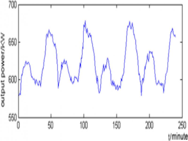
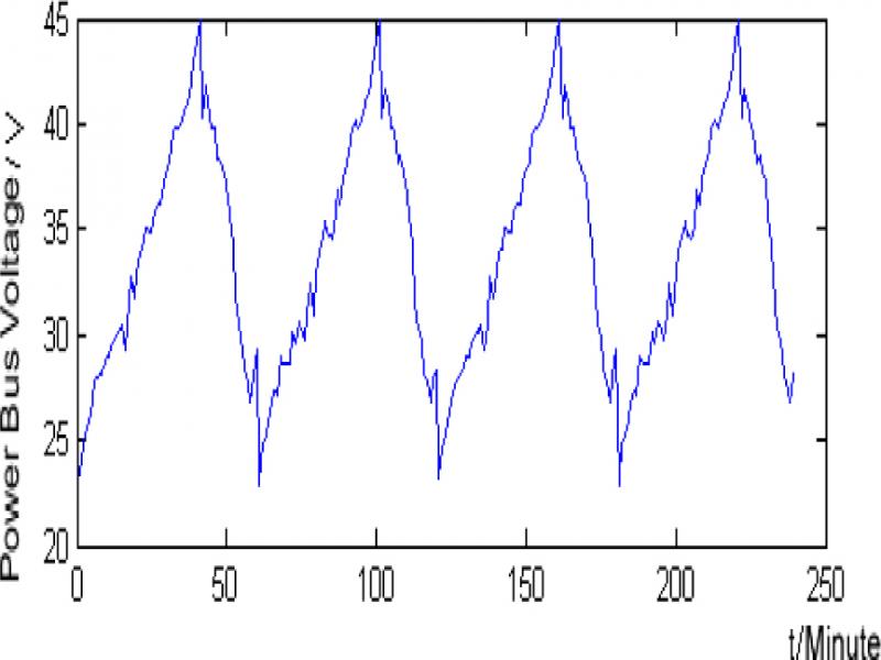
Telemetry data has the characteristics of non-stationary variation, commonly used statistics of the telemetry data (such as the mean and autocorrelation function, etc.) often varies with time changing, it bring very great difficulty to the telemetry data forecast. Through the telemetry data 1 and 2 (table 1, 2) statistics, difference is very big, every stage of the statistical parameters show that the sequence of non-stationary time series. Wavelet analysis to deal with this kind of data has a great advantage.

TABLE I.

THE TEST RESULTS OF A REMOTE SENSING DATA 1 STATIONARITY

TABLE II.

THE TEST RESULTS OF A REMOTE SENSING DATA 2 STATIONARITY

Time	24	60	120	240
Mean Value	608.618	620.9572	622.6287	622.6287
Variance	198.2080	604.1601	611.2902	674.6010

Figures 1, 2 is telemetry data 1 and 2 for four hours of change curve, it can be seen that the output power sequence is periodicity, as well as randomness. The coexistence of periodicity and randomness, the result can be seen as the superposition of different frequency components, these frequency components superimposed on each other in the interior have similar frequency characteristics and the same variation. If the subsequence to establish a prediction model for single change, due to the change of the data characteristics of a single, reduce the difficulty of forecasting model selection.

Data of 1 consecutive 4 hours curve graph

Data of 2 consecutive 4 hours curve graph

B. The choice of wavelet function

There are some mutations in the trend of spacecraft telemetry data, and these mutations reflect the actual state of the satellite. In order to accurately capture the point of the mutation, the wavelet function is usually required to have a fast convergence, which can quickly attenuate to zero^[5]. In this paper, db3 wavelet is chosen as the wavelet base for the different scale of a certain remote data sequence. DbN wavelet in N=1, 3, 4, 1, the results of 2 scale decomposition of a telemetry data (Figure 3).

Comparison results of dbN wavelet based N=1,2,3,4

The choice of wavelet function can satisfy the following 3 conditions except that the condition and the regularity condition^[2].

1) Good compact support;
2) ψ(t) has vanishing moments; vanishing moments can make the wavelet function has a good locality in the frequency domain;
3) Satisfy orthogonality.

C. Wavelet decomposition scale study

Due to the telemetry data is not stable, its change cycle is difficult to see, and its change is slow and fast change together, that is, the change of telemetry data cycle is the size of the cycle of nested together. Therefore, Separating different frequency component can make its change rule is more intuitive, and can also improve data non-stationary^[6]. The figure 4 Show the results that comparison db3 wavelet approximation part aN decomposed at different scales and a0 of the original sequence.

Comparison of different decomposition scale approximation section

It can be seen that the decomposition scale is 2, the curve of the approximate part a2 has smooth enough, and basically maintained the shape of the original curve, while A3, A4, because of the increase in the number of points, the sampling point is reduced, the approximate partial curve is too smooth, the sequence of changes in the trend has been distorted, so this paper chose the decomposition of 2.

D. Forecasting model of time series

Time series forecasting^[3][7] is one of the methods of statistical analysis. Its modeling idea is the basic assumption that the change of the past of the telemetry data will continue into the future, that is, the future is a continuation of the past. In this paper, the use of the periodic autoregressive model (PAR model)^[8][9] is as follows:

If there is a time series X, the expression is

(9)

X_{t} = a_{0 t} + a_{1, t} X_{t - 1} + a_{2, t} X_{t - 2} + \dots + a_{p, t} x_{t - p} + ϵ_{t}

Meet the following conditions:

1) ε_t is independent sequence, Expected Value is Eε_t = 0, variance is ${E ϵ}_{t}^{2} = σ_{t}^{2}$ ;
2) For any i = 0,1,…,p, a_it = a_it+T, $σ_{t}^{2} = σ_{i t + T}^{2}$ , t = 0,±1,…, among T is a positive number, and the model is model of PAR, T is the Cycle length of PAR model, t is phase of PAR model.

The forecast model of the telemetry data is:

\begin{array}{l} X_{K T + 1} = a_{01} + a_{11} X_{K T} + \dots + a_{γ 1} X_{K T + 1 - γ} + ϵ_{K T + 1} \\ X_{K T + 2} = a_{2} + a_{2} X_{K T + 1} + \dots + a_{γ 2} X_{K T + 2 - γ} + ϵ_{K T + 2} \\ \dots \dots \\ X_{K T + T} = a_{0 T} + a_{1 T} X_{K T + T - 1} + \dots + a_{γ T} X_{K T + T - γ} + ϵ_{K T + T} \end{array}

Set X₁, X₂,…, X_n is telemetry data samples of per minute, the value of X_t(h) in the future h is the X_t+h in the condition of t, and thus as its predictive value, denoted as ${\hat{X}}_{n} (t)$ , according to the definition of:

Decomposition for telemetry data sequence prediction model is established for an hour, the selection of the length of the cycle is 60, namely, p=T=60. This load sequence PAR prediction model can be represented by the expression of the following:

\begin{array}{l} {\hat{X}}_{n} (k) = a_{k T, k} + a_{k T + 1, k} {\hat{X}}_{n} (k - 1) + \dots + a_{k T + 60, k} {\hat{X}}_{n} (k - 60) \\ \begin{matrix} a_{k T + i, k} & (i, k = 1, 2, \dots, 60) \end{matrix} \end{array}

E. Predicted results analysis

The predicted values of the reconstructed sub sequences of the scales are compared with the original output power trends (Figure 5).

Comparison results between predicted values and actual results

By analyzing the comparison between an actual telemetry data and the predicted value, it can be seen that the boundary of the predicted results and the trend of mutation is not very ideal. In this paper, the extension of the periodic continuation to the boundary of the sequence is extended. The idea of periodic continuation is that the signal is considered as a periodic signal, and the extension process is as follows^[10][11]:

{\begin{matrix} x_{n} = x_{n + M}, & n < 0 \\ x_{n} = x_{n - M}, & n < M < 1 \end{matrix}

Among, M is the length of sequence. The comparison result of the prediction curve and the actual curve after eliminating the boundary error is shown in Figure 6.

The comparison results between the predicted values and the actual values of the modified boundary

From Figure 6, we can see that the results of the prediction of the sequence are better than the results obtained by the wavelet transform.

IV. THE PERFORMANCE EVALUATION OF THE TELEMETRY DATA FORECASTING MODEL

Thought of optimal decision method is using linear transform to normalize the attribute value, and at the same time using the ideal point and negative ideal point, compared with the traditional method has more rationality and reliability. The ideal point is the best solution, and its target value is the best, the worst is the worst. The worst is the worst. The optimal solution algorithm is as follows:

A. Set decision matrix of A is

(10)

A = \begin{matrix} f_{1} (x) \\ f_{2} (x) \\ ⋮ \\ f_{p} (x) \end{matrix} [\begin{matrix} f_{1} (x_{1}) & f_{1} (x_{2}) & \dots & f_{1} (x_{n}) \\ f_{2} (x_{1}) & f_{2} (x_{2}) & \dots & f_{2} (x_{n}) \\ ⋮ & ⋮ & ⋮ & ⋮ \\ f_{P} (x_{1}) & f_{P} (x_{2}) & \dots & f_{P} (x_{n}) \end{matrix}]

(11)

\underset{- i}{U} = \min (f_{i} (x_{1}), f_{i} (x_{2}), \dots, f_{i} (x_{n})}, i = 1, 2, \dots, k

\begin{array}{l} {\bar{U}}_{i} = \max (f_{i} (x_{1}), f_{i} (x_{2}), \dots, f_{i} (x_{n})}, i = k + 1, k + 2, \dots, P \\ {\bar{V}}_{i} = \max (f_{i} (x_{1}), f_{i} (x_{2}), \dots, f_{i} (x_{n})}, i = 1, 2, \dots, k \\ \underset{- i}{V} = \min (f_{i} (x_{1}), f_{i} (x_{2}), \dots, f_{i} (x_{n})}, i = k + 1, k + 2, \dots, P \end{array}

B. To determine the ideal point and negative ideal point

The ideal point:

(12)

x^{*} = {({\underline{U}}_{1}, {\underline{U}}_{2}, \dots, {\underline{U}}_{k}, {\bar{U}}_{k + 1}, {\bar{U}}_{k + 2}, \dots, {\bar{U}}_{P})}^{T}

Negative ideal point:

\bar{x} = {({\bar{V}}_{1}, {\bar{V}}_{2}, \dots, {\bar{V}}_{k}, {\underline{V}}_{k + 1}, \dots, {\underline{V}}_{P})}^{T}

C. Calculate the close degree

The proximity of the ideal point

(13)

R_{i} = \frac{1}{P} [Σ_{j = 1}^{k} \frac{{\underline{U}}_{j}}{f_{j} (x_{i})} + Σ_{j = k + 1}^{p} \frac{f_{j} (x_{i})}{{\bar{U}}_{j}}], i = 1, 2, \dots, n

The proximity of the negative ideal point

(14)

r_{i} = \frac{1}{P} [Σ_{j = 1}^{k} \frac{f_{j} (x_{i})}{{\bar{V}}_{j}} + Σ_{j = k + 1}^{p} \frac{{\underline{V}}_{j}}{f_{j} (x_{i})}], i = 1, 2, \dots, n

D. Calculate the relative close degree

(15)

ϵ_{i} = \frac{R_{i}}{r_{i} + R_{i}}, 0 \leq ϵ_{i} \leq 1, i = 1, 2, \dots, n

By calculating the formula (1) (11) (12) is as follows:

The ideal point:

x^{*} = {({\underline{U}}_{1}, {\underline{U}}_{2}, \dots, {\underline{U}}_{k}, {\bar{U}}_{k + 1}, {\bar{U}}_{k + 2}, \dots, {\bar{U}}_{P})}^{T} = (1.23, 0.978, 4.219, 1.491)

Negative ideal point:

\bar{x} = {({\bar{V}}_{1}, {\bar{V}}_{2}, \dots, {\bar{V}}_{k}, {\underline{V}}_{k + 1}, \dots, {\underline{V}}_{P})}^{T} = (3.76, 3.679, 7.896, 4.118)

Calculate the relative close degree by the formula (13) (14) (15): ε =0.34

From the relative closeness of view, the time series forecasting model program has a higher rationality and reliability.

V. CONCLUSION

This paper studies the telemetry data forecasting method based on wavelet analysis. Through the analysis of the characteristics of the telemetry data, the characteristics of the non - stationary and certain periodicity of the telemetry data are established, and the prediction algorithm based on wavelet analysis is established. By choosing different wavelet bases and the decomposition scale, the decomposition results show that 2, db3 wavelet decomposition scale is the best. Based on the Mallat algorithm, the time series forecasting model is established according to the characteristics of detail data and approximate data. The experimental results show that the predicted values are in good agreement with the actual values. Finally, through the analysis of the performance of the forecasting model, the forecasting model is reasonable and reliable.

Time	24	60	120	240
Mean Value	29.2479	35.413	37.1234	39.2378
Variance	10.3366	30.9019	37.4902	42.5010

Application of Wavelet Analysis in The Prediction of Telemetry Data

Full Article

I. INTRODUCTION

II. WAVELET ANALYSIS THEORY

A. Wavelet analysiss

(1)

(2)

B. Mallat algorithm

1). Mallat algorithm based on wavelet decomposition

(3)

(4)

(5)

(6)

(7)

2). Reconstruction algorithm of mallat algorithm

(8)

III. THE RESEARCH OF TELEMETRY DATA TIME SERIES PREDICTION BASED ON MALLAT ALGORITHM

A. The characteristics of telemetry data

TABLE I.

TABLE II.

Figure 1.

Figure 2.

B. The choice of wavelet function

Figure 3.

C. Wavelet decomposition scale study

Figure 4.

D. Forecasting model of time series

(9)

E. Predicted results analysis

Figure 5.

Figure 6.

IV. THE PERFORMANCE EVALUATION OF THE TELEMETRY DATA FORECASTING MODEL

A. Set decision matrix of A is

(10)

(11)

B. To determine the ideal point and negative ideal point

(12)

C. Calculate the close degree

(13)

(14)

D. Calculate the relative close degree

(15)

V. CONCLUSION