
Table 1
Analytic interfaces used in this study
| Version | Source | |
|---|---|---|
| UCINET | 6.564 | http://www.analytictech.com/ |
| Pajek | 4.03 | http://pajek.imfm.si/ |
| ORA-NetScenes | 3.0.9.9.20 | http://www.casos.cs.cmu.edu/projects/ora/ |
| Gephi | 0.8.2 | http://gephi.org/ |
| sna | 2.3-2 | http://www.statnet.org/ |
| igraph | 0.7.1 | http://igraph.org/ |
Table 2
Output scaling
| Degree | Closeness | Betweenness | Eigenvector | |
|---|---|---|---|---|
| Gephi | Raw | Normalized Average | Raw | Scaled (max=1) |
| Pajek | Raw | Normalized | Normalized | Normalized |
| UCINET | Raw | Average | Raw | Normalized |
| ORA | Normalized | Normalized | Normalized | Normalized |
| sna | Raw | Normalized | Raw | Normalized |
| igraph | Raw | Normalized | Raw | Scaled (max=1) |
Table 3
Data used for reliability comparisons
| Data | Nodes in Main Component | Nodes in Smaller Components | Number of Loops | Max. Number of Nodes | Average Degree |
|---|---|---|---|---|---|
| Small One-mode | 29 | 6 | 6 | 35 | 3.5 |
| Large One-mode | 1876 | 112 | 60 | 2000 | 3.0 |
| Small Two-mode | (10, 21) | 4 | NA | (10, 25) | 3.7 |
| Large Two-mode | (300, 1815) | 185 | NA | (300, 1700) | 3.7 |
Table 4
Consistency of output by centrality type and network conditions
| No Disconnected Components & No Loops | Disconnected Components | Loops | Disconnected Components Loops | |||||
|---|---|---|---|---|---|---|---|---|
| 1 Mode | 2 Mode | 1 Mode | 2 Mode | 1 Mode | 2 Mode | 1 Mode | 2 Mode | |
| Betweenness Centrality | High | High | High | High | High | NA | High | NA |
| Degree Centrality | High | Medium | High | Medium | Low | NA | Low | NA |
| Eigenvector Centrality | Medium | Medium | Medium | Low | Medium | NA | Low | NA |
| Closeness Centrality | Medium | Medium | Low | Low | Medium | NA | Low | NA |
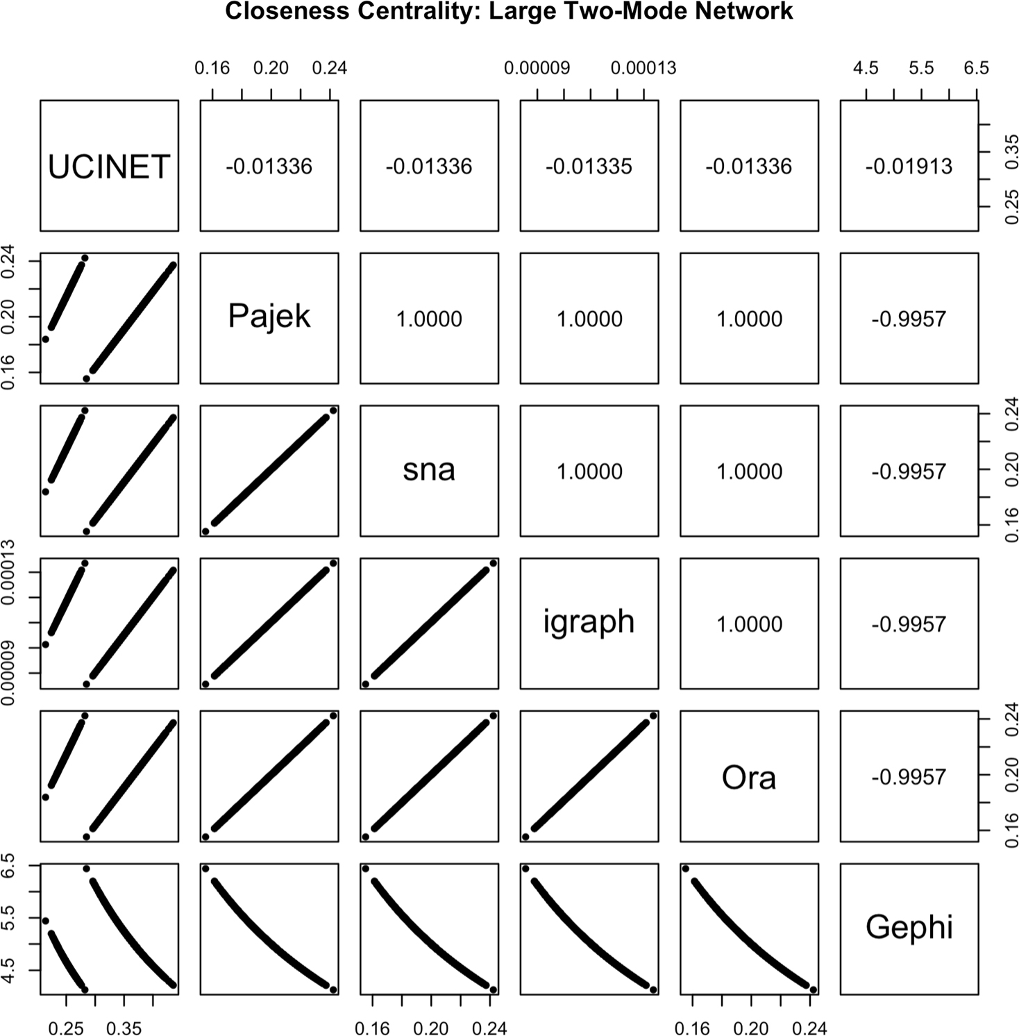
Figure 1
Scatterplot matrix comparing closeness centrality output for a large, two-mode network. Pearson’s correlation coefficients between programs are provided above the diagonal.
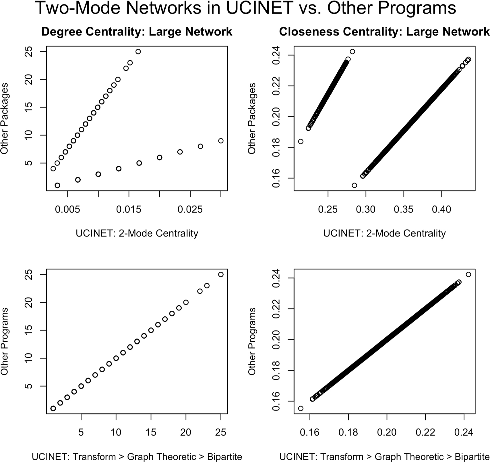
Figure 3
A variety of solutions are possible when analyzing two-mode networks in UCINET. Top Row: Scatterplots of UCINET’s degree (r = 0.3713) and closeness (r = -0.0134) output using the two-mode centrality procedure, compared with other analytic packages. All other packages performed identically. Bottom Row: When transformed into a bipartite network format, UCINET calculates as for a one-mode network, and results are analogous to other packages. Closeness centrality for the bipartite aspect was calculated using Freeman normalization in UCINET.
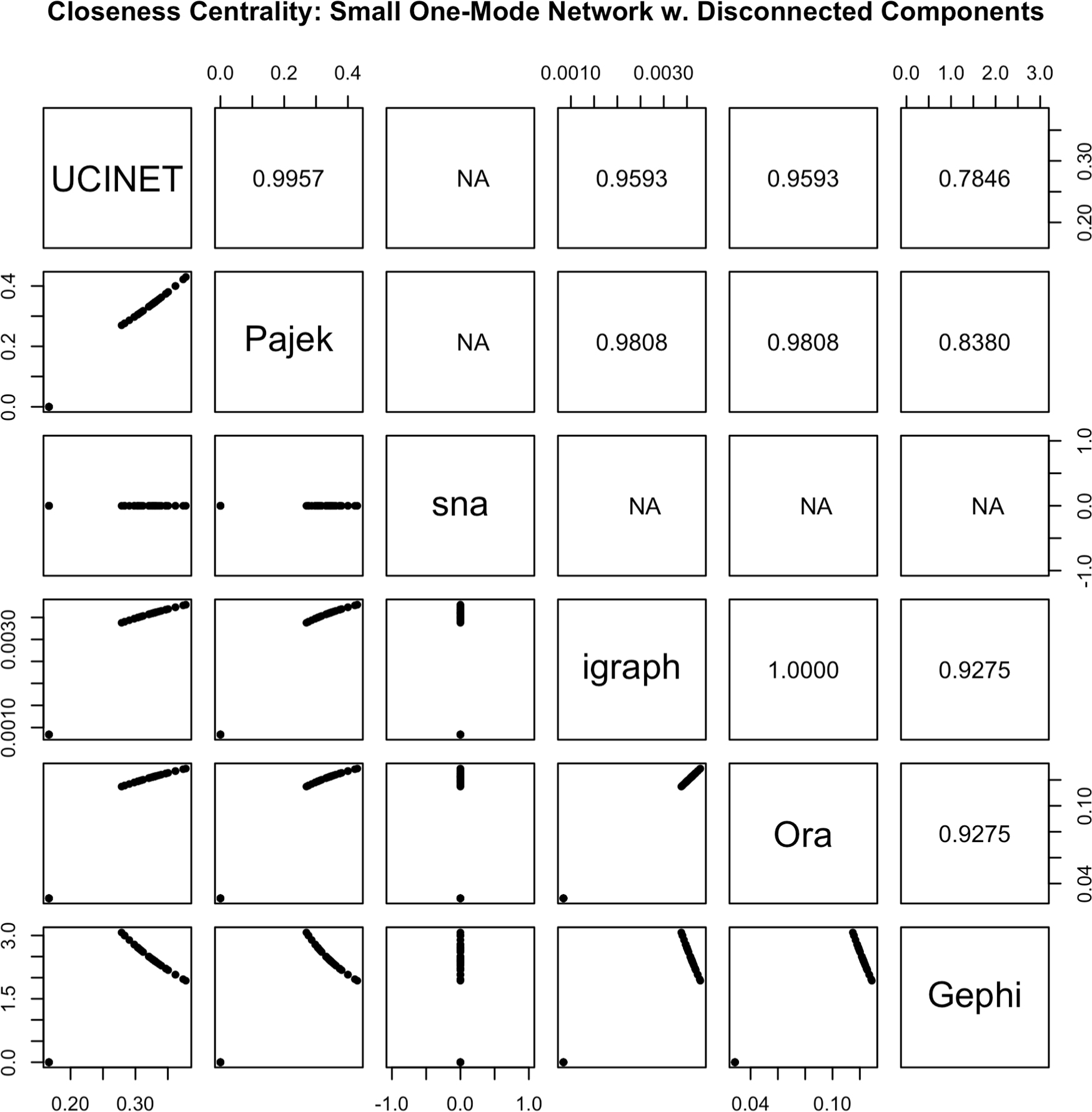
Figure 2
Scatterplot matrix comparing output for closeness centrality in a small, one-mode network. Pearson’s correlation coefficients between programs are provided above the diagonal. Note that the sna package for R does not produce measures between disconnected components, resulting in correlation values listed as “NA”.
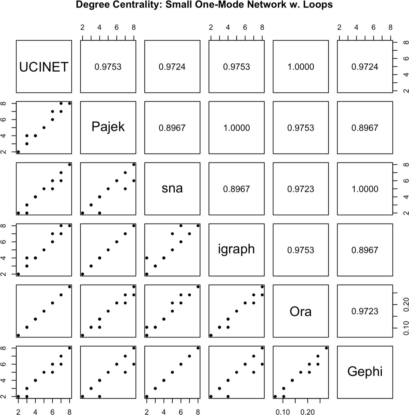
Figure 4
Scatterplot matrix comparing degree centrality output for a small, one-mode network containing loops. Pearson’s correlation coefficients between programs are provided above the diagonal.
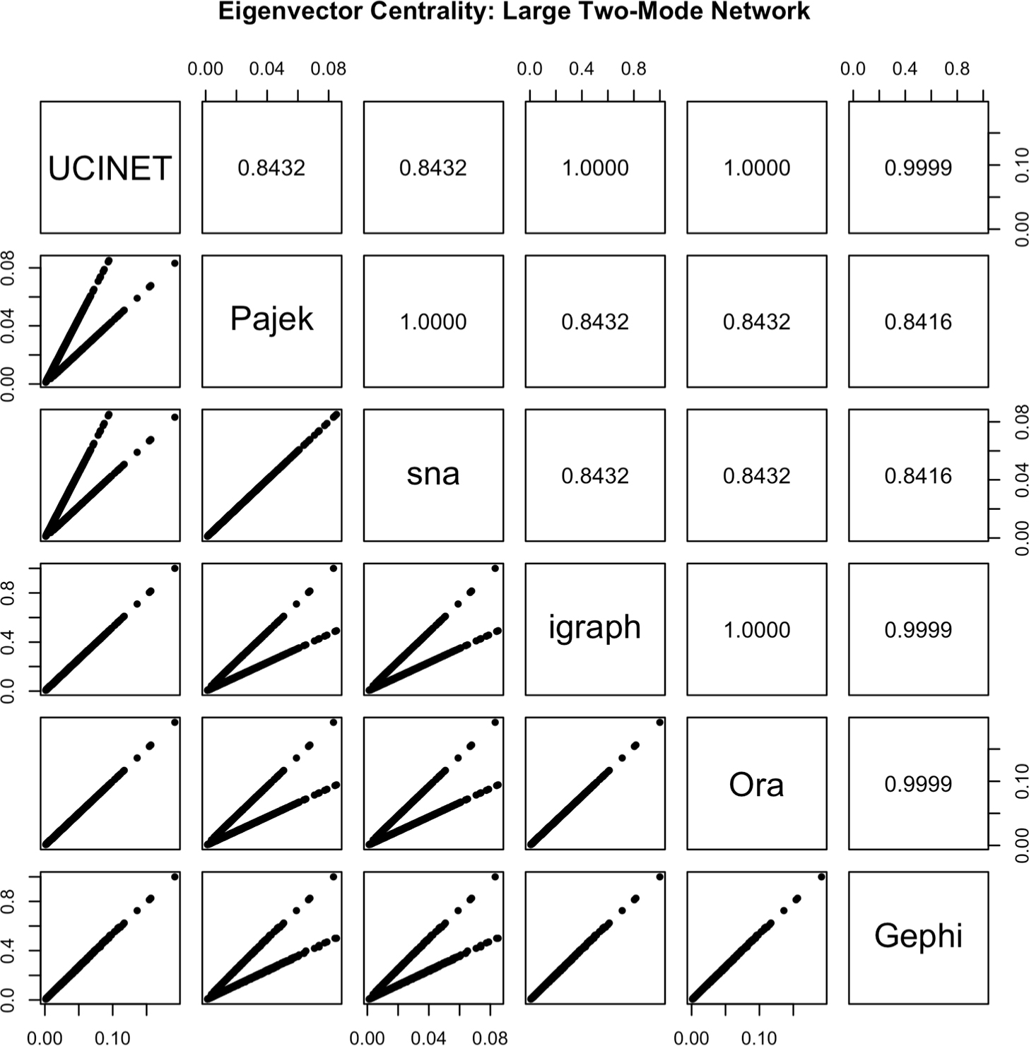
Figure 5
Scatterplot matrix comparing eigenvector centrality output for a large, two-mode network. Pearson’s correlation coefficients between programs are provided above the diagonal. Pajek output for this plot was calculated using “important vertices”, a two-mode generalization of hubs and authorities.
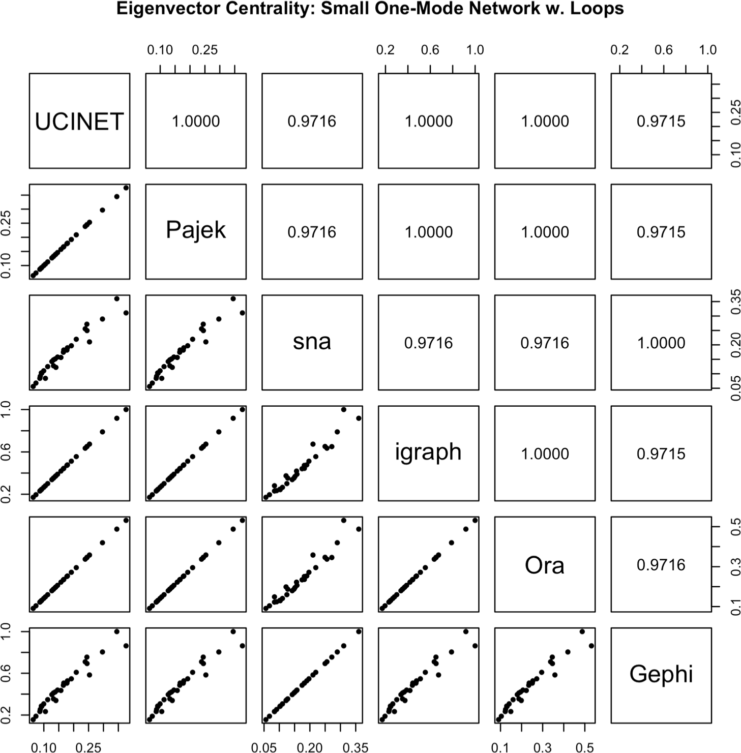
Figure 6
Scatterplot matrix of eigenvector centrality output for a small, one-mode network with loops. Pearson’s correlation coefficients between programs are provided above the diagonal. Note, initial calculations in sna – shown above – were run using the default argument (diag=FALSE). For additional variation, consult the text above.
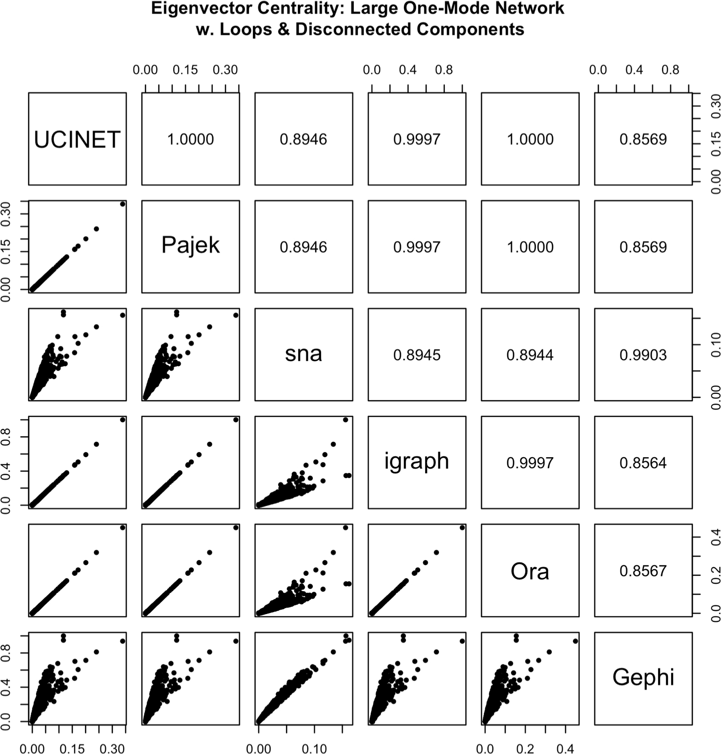
Figure 7
Scatterplot matrix comparing eigenvector centrality output for a moderately large, one-mode network containing loops and disconnected components. Pearson’s correlation coefficients between programs are provided above the diagonal.
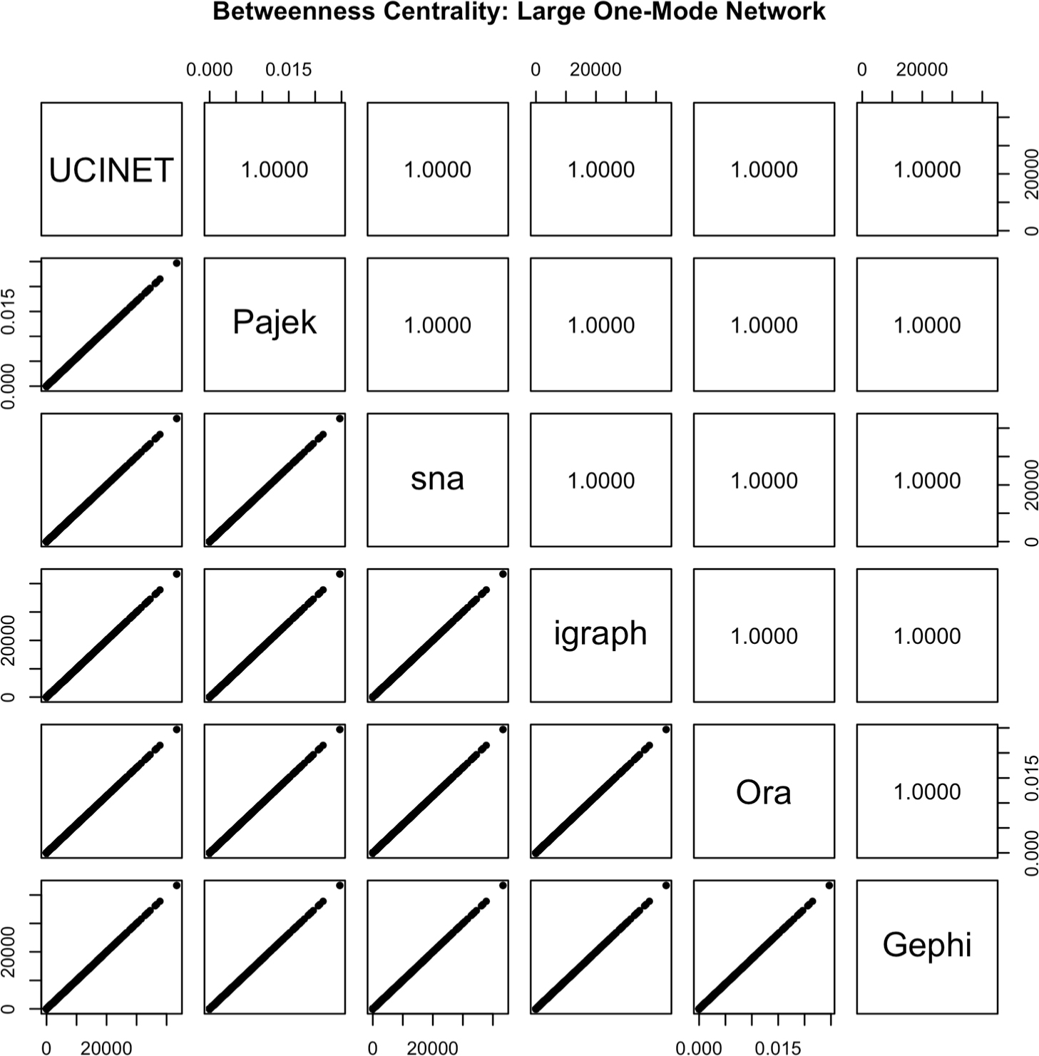
Figure 8
Scatterplot matrix comparing betweenness centrality output for a large, one-mode network. Pearson’s correlation coefficients between programs are provided above the diagonal.
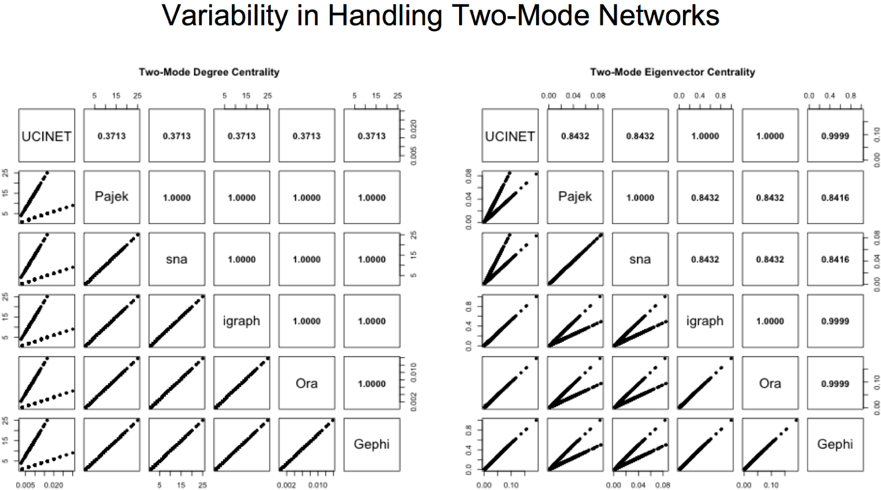
Figure 9
Scatterplot matrices comparing degree and eigenvector output for a two-mode network. Neither network contains loops or disconnected components. Pearson’s correlation coefficients between programs are provided above the diagonal.