
Table 1.
Parameters of outdoor air – summer conditions
| Climatic zone | Maximum temperature, relative humidity, equivalent solar load |
|---|---|
| I | 40°C, 40%, 800W/m2 |
| II | 35°C, 50%, 700 W/m2 |
| III | 28°C, 45%, 600W/m2 |
Table 2.
Parameters of outdoor air – winter conditions
| Climatic zone | Minimal temperature |
|---|---|
| I | -10°C |
| II | -20°C |
| III | -40°C |
Table 3.
The minimum total volume flow of fresh air for railway vehicles with air conditioning device
| Exterior temperature (t em ) | Minimum fresh air rate equivalent to +20°C and 50% rel. hum, normal atmospheric pressure |
|---|---|
| t em < -15°C | 10m3/h /passenger |
| -15°C ≤ t em ≤ -5°C | 15m3/h /passenger |
| -5°C ≤ t em ≤ +26°C | 20m3/h /passenger |
| t em > 26°C | 15m3/h /passenger |
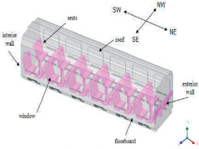
Figure 1.
The numerical coach model – geometry
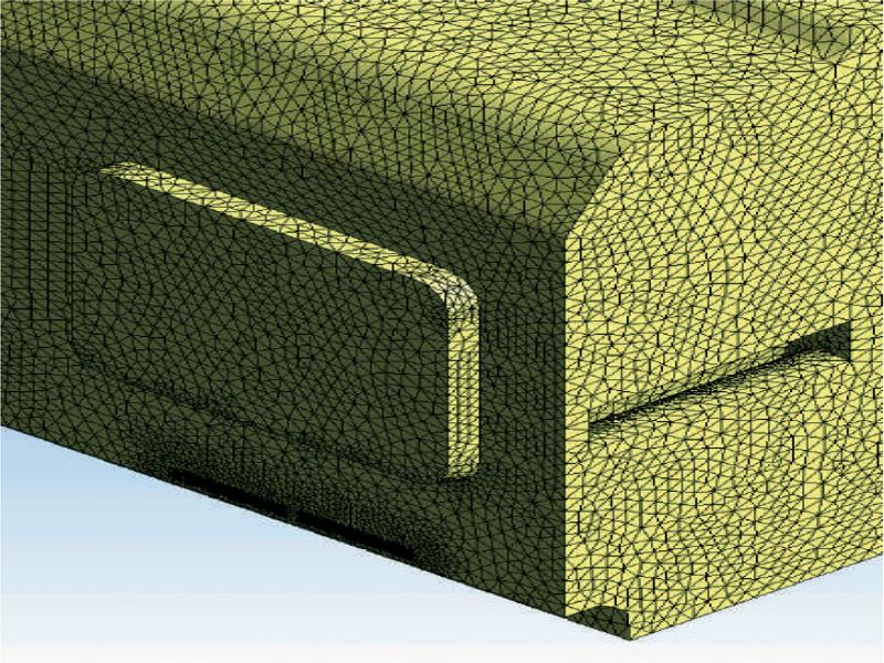
Figure 2.
The discretization grid on the side of the exterior partitions of the coach
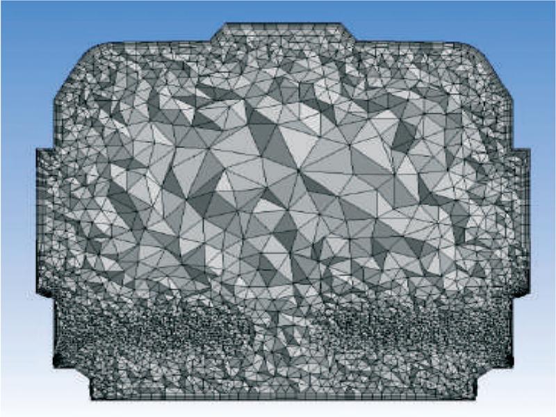
Figure 3.
The discretization grid with inflated boundary – the crosssection
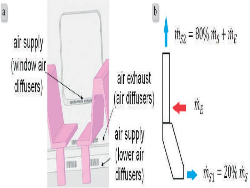
Figure 4.
a) Localization of diffusers, b) scheme of air distribution in the coach, – mass flow rate of air supply – mass flow rate of air supply by lower air diffusers, – mass flow rate of air supply by window air diffusers, – mass flow rate of air exhaust
Table 4.
Boundary conditions for case 1
| The element of model and kind of boundary conditions | Value of case 1 |
|---|---|
| South-east wall; “Wall” with heat transfer coefficient U and sol-air temperature | |
| Interior wall; “Wall” | Adiabatic wall |
| North-west wall; “Wail” with heat teansfer coefficient U and sol-air temperature | |
| North-east wall; “Wall” with heat transfer coefficient U and sol-air temperature | |
| South-east windows; “Wall” with heat transfer coefficient U and sol-air temperature | |
| North-west windows; “Wall” with drat transfer coefficient U and sol-ars temperature | |
| Roof; “Well” with heat transfer coefficienit U and sol-air temperature | |
| Floorboard; “Well” with heat transfer “coefficient U and exterior-temperature | |
| Lower diffusers; “Inlet” with mass flow rale of supply air and temperature of ventilation supply air | |
| Upper diffusers; "Inlet” with mass flow rate of supply air and temperature of ventilation supply air | |
| Exhaust diffusers; “Outlet” wish mass flow rate of exhaust air |
Table 5.
Boundary condition for case 2
| The element of model and kind of boundary conditions | Value of case 2 |
|---|---|
| South-east wall; “Wall” with heat transfer coefficient U and sol-a ir temperature | |
| Interior wall; “Wall” | Adiabatic wall |
| North-west wall; “Wall” with heat tran sfer coefficient U and sol- air temperature | |
| North-east wall; “Wall” with heat transfer coefficient U and sol-air temperature | |
| South-east windows; “Wall” with heat tr ansfer coeffi cient U and sol-a ir temperature | |
| North-west windows; “Wall” with heat transfer coeffi cient U and sol-air temperature | |
| Roof; “Wall” with heat tr ansfer coefficient U and sol-air temperature | |
| Floorboard; “Wall” wi th heat transfer coefficient U and exterior temperature | |
| Lower diffusers; “Inlet” with mass flow rate of supply air and temperature of ventilation supply air | |
| Upper diffusers; “Inlet” with mass flow rate of supply air and temperature of ventilation supply air | |
| Exhaust diffusers; “Outlet” with mass flow rate of exhaust air |
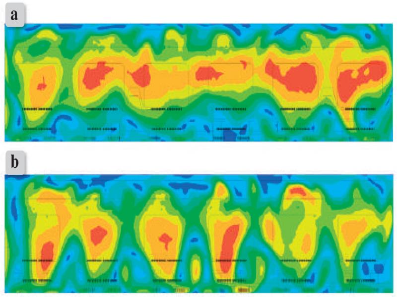
Figure 5.
The comparison of distribution of air velocity in the vertical plane XY, Z = 1.804 m: a) case 1, b) case 2
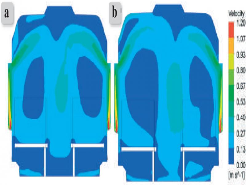
Figure 6.
The comparison of the distribution of air velocity in the vertical plane YZ, X = -11.63 m: a) case 1, b) case 2
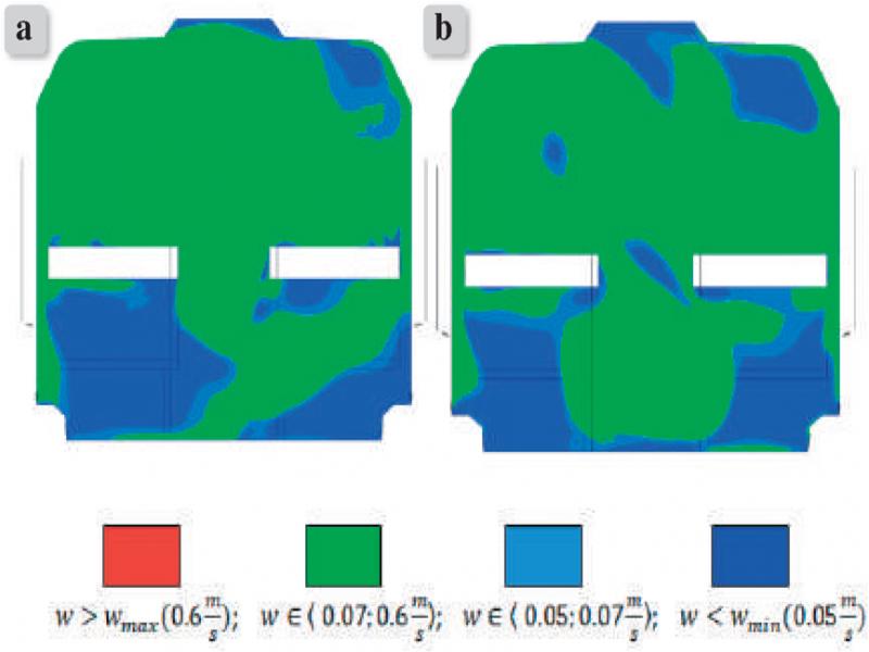
Figure 7.
The comparison of the comfort zone in the vertical plane YZ, X= -9.55 m: a) case 1, b) case 2
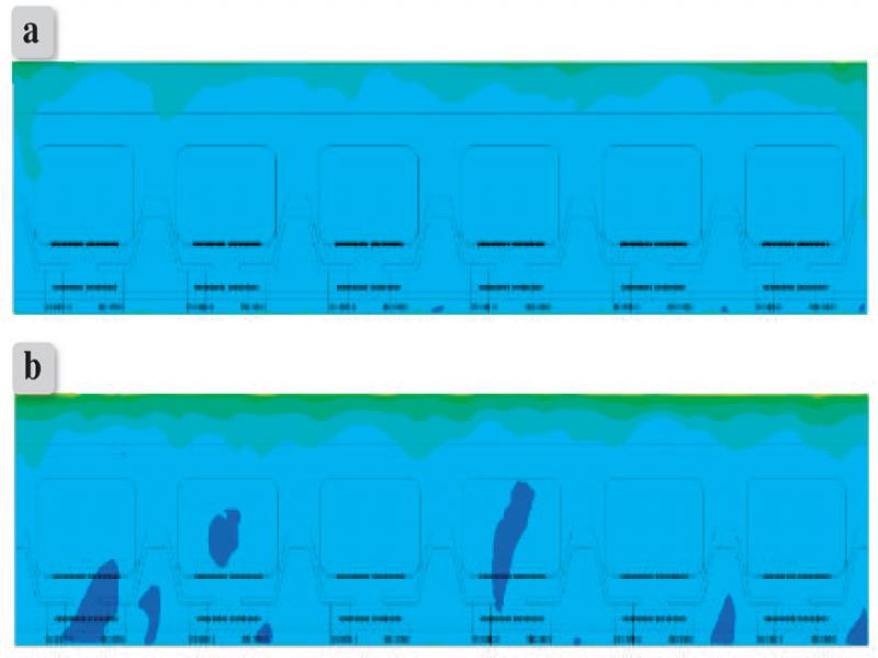
Figure 8.
The comparison of the distribution of air temperature in the vertical plane XY, Z = 1.804 m: a) case 1, b) case 2
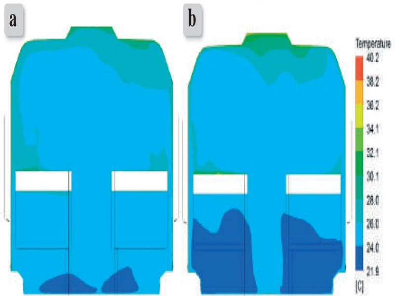
Figure 9.
The comparison of the distribution of air velocity in the vertical plane YZ, X = -9.55 m: a) case 1, b) case 2
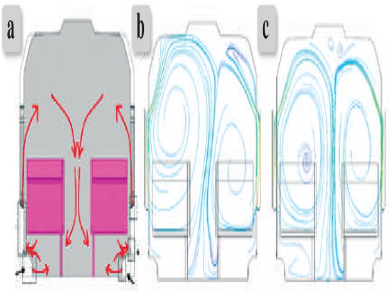
Figure 10.
The comparison of the distribution of air velocity in the vertical plane YZ, X = -11.63 m: a) theoretical distribution, b) numerical distribution for case 1, c) numerical distribution for case 2
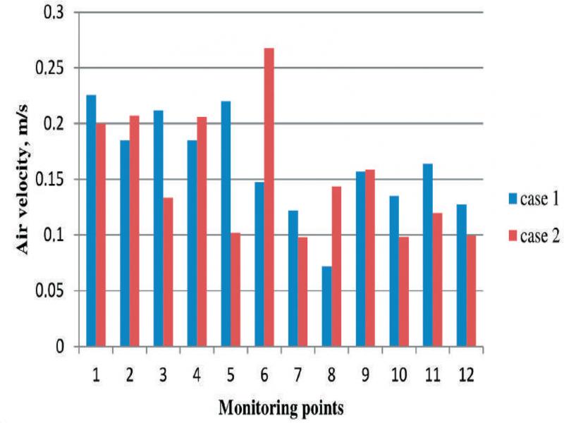
Figure 11.
The comparison of air velocity in monitoring points for case 1 and case 2
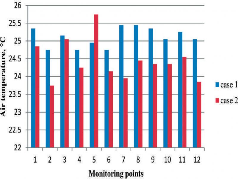
Figure 12.
The comparison of air temperature in monitoring points for case 1 and case 2