
Table 1:
Count of government types in Georgia, 2015.
| Government Type | # of entities | Government Type | # of entities |
|---|---|---|---|
| County | 152 | Special Purpose | 1141 |
| City-County Consolidations | 7 | Airport | 44 |
| City | 531 | Building | 38 |
| Development | 235 | ||
| Downtown Development | 207 | ||
| Hospital | 112 | ||
| Housing | 165 | ||
| Industrial Development | 43 | ||
| Joint Development | 52 | ||
| Public Facilities | 21 | ||
| Recreation | 18 | ||
| Solid Waste | 28 | ||
| Tourism | 20 | ||
| Urban Redevelopment | 33 | ||
| Water and Sewer | 64 | ||
| Other | 61 |
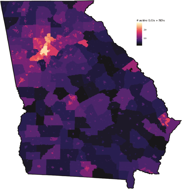
Figure 1:
Density of general and special purpose governments in Georgia, 2015.
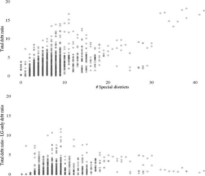
Figure 2:
Aggregate local public debt over total assessed property value by county, 2005–2014.
Table 2:
Summary of explanatory variables.
| County×Year | Mean | St. Dev. | Min | Median | Max | |
|---|---|---|---|---|---|---|
| Total Districts | 159×10 | 7.27 | 4.95 | 0 | 6 | 42 |
| Multi-jurisdictional Districts | 159×10 | 2.47 | 1.49 | 0 | 2 | 10 |
| Single-jurisdictional Districts | 159×10 | 4.80 | 4.23 | 0 | 4 | 32 |
| Independent Districts | 159×10 | 5.04 | 3.46 | 0 | 4 | 31 |
| Dependent Districts | 159×10 | 2.23 | 2.28 | 0 | 2 | 15 |
| SD/SD+LG Operating Expense Ratio | 159×10 | 0.21 | 0.24 | 0.00 | 0.10 | 0.93 |
Table 3:
Summary of control variables.
| County×Year | Mean | St. Dev. | Min | Median | Max | |
|---|---|---|---|---|---|---|
| Population (10k) | 159×10 | 6.043 | 12.655 | 0.167 | 2.259 | 99.646 |
| Yearly pop. growth (%) | 159×10 | 0.710 | 1.868 | −16.090 | 0.568 | 12.417 |
| % pop. over age 65 | 159×10 | 13.715 | 3.749 | 2.618 | 13.557 | 32.263 |
| % pop. with Bachelor’s | 159×10 | 4.041 | 3.322 | 0.000 | 3.300 | 23.500 |
| % households with children | 159×10 | 30.145 | 6.099 | 12.144 | 29.750 | 56.464 |
| Unemployment % | 159×10 | 8.395 | 3.024 | 3.000 | 8.250 | 22.900 |
| Income per capita (1k) | 159×10 | 28.546 | 6.220 | 14.127 | 27.535 | 64.877 |
| Rural-Urban Continuum: | Metro: 44.5% | Suburban: 39.6% | Rural: 15.9% | |||

Figure 3:
95% credible intervals for linear covariates testing H1 – H3 (models also include random effects for time, county, and spatial correlation).
Table A1:
Tabular parameter estimates for models shown in Figure 3.
| Total Districts | District Jurisdiction | District Status | |
|---|---|---|---|
| Population (10k) | −0.014 (−0.036, 0.008) | −0.014 (−0.036, 0.007) | −0.016 (−0.038, 0.007) |
| Yearly population growth % | 0.024 (−0.014, 0.063) | 0.025 (−0.014, 0.064) | 0.025 (−0.014, 0.064) |
| % pop. over age 65 | 0.011 (−0.040, 0.062) | 0.011 (−0.041, 0.062) | 0.012 (−0.040, 0.064) |
| % households w/children | 0.026 (−0.000, 0.052) | 0.026 (−0.000, 0.052) | 0.026 (−0.000, 0.052) |
| Unemployment % | −0.018 (−0.040, 0.005) | −0.018 (−0.041, 0.004) | −0.018 (−0.040, 0.004) |
| Income per capita ($1k) | 0.002 (−0.025, 0.029) | 0.002 (−0.025, 0.029) | 0.003 (−0.024, 0.030) |
| % pop. with degree | −0.001 (−0.001, 0.000) | −0.001 (−0.001, 0.000) | −0.001 (−0.001, 0.000) |
| Rural | −0.556 (−1.089, −0.022) | −0.554 (−1.087, −0.020) | −0.556 (−1.089, −0.022) |
| Suburban | −0.144 (−0.541, 0.254) | −0.142 (−0.540, 0.256) | −0.132 (−0.531, 0.267) |
| SD Operating Expenses ($1M) | 0.004 (0.003, 0.006) | 0.004 (0.003, 0.005) | 0.004 (0.003, 0.005) |
| # local governments | −0.008 (−0.093, 0.078) | −0.008 (−0.093, 0.077) | −0.008 (−0.094, 0.077) |
| # special districts | 0.111 (0.069, 0.153) | ||
| # single-juris. SDs | 0.122 (0.071, 0.173) | ||
| # multi-juris. SDs | 0.086 (0.008, 0.163) | ||
| # dep. SDs | 0.117 (0.057, 0.176) | ||
| # ind. SDs | 0.109 (0.062, 0.156) |
*Posterior mean (0.025, 0.975 quantiles).
Table A2:
Random effect coefficient estimates for models shown in Figure 3.
| Total | Jurisdiction | Status | |
|---|---|---|---|
| Precision for the Gaussian observations | 0.033 (−0.006, 0.338) | 0.033 (−0.006, 0.332) | 0.033 (−0.006, 0.337) |
| Precision for Year | 0.822 (0.635, 1.037) | 0.820 (0.634, 1.036) | 0.823 (0.638, 1.044) |
| Rho for Year | 1933.578 (127.764, 6841.167) | 1858.089 (128.302, 6716.727) | 1788.939 (125.042, 6591.693) |
| Group Rho for Year | 18079.047 (1221.672, 66239.178) | 17489.928 (1189.490, 65241.233) | 18352.315 (1249.464, 66756.094) |
| Precision for county (iid component) | 0.887 (0.823, 0.954) | 0.887 (0.823, 0.954) | 0.886 (0.823, 0.953) |
| Precision for county (spatial component) | 0.018 (−0.988, 0.987) | 0.013 (−0.988, 0.987) | 0.009 (−0.987, 0.987) |
*Posterior mean (0.025, 0.975 quantiles).
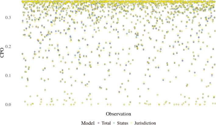
Figure A1:
CPO values for each model plotted against observations.