
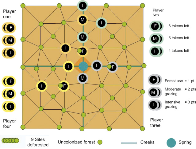
Figure 1
The Sierra Springs game board and tokens. The board has 48 forested land units (green tokens) that can be colonized. Each player gets six tokens each for the three land uses, and has access to a quadrant of the territory. Quadrants are separated by creeks. Within a quadrant, 8 inner land units are available only to the owner, while 8 border land-units (shared with two other players) will be owned by the neighbor who first colonizes them. In the figure, each player has selected 3 locations and placed 3 tokens on the board. Nine sites have been deforested and thereby, their forest tokens removed. Land use tokens have been placed to show examples of problematic situations: player 2 – as well as players 1 and 4 – have contiguous Is; players 1 and 2 have damaged their common creek; players 3 and 4 have damaged the community’s spring.
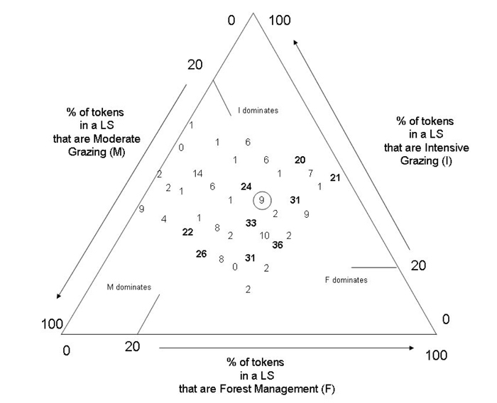
Figure 2
Each possible local solution (LS) on, say, quadrant 1 is a [F, M, I] triad which can be described by its (percentual) proportions of F, M and I tokens, and by its Pj values (i.e. the percentage of the 704 global solutions (GS’s) with which that triad is compatible). For example, the triad [4, 6, 3], is made of 31% F, 46% M, and 23% I, and it occurs in 9% of the GS’s. Both attributes of this triad can be mapped on the ternary plot above (see circled number). The position of the circle represents the percentages of F, M, and I tokens in the triad, while the number inside it represents its Pj value. All 37 LS available to a player are similarly mapped on the plot, but the circles have been excluded to avoid crowding the figure. “Easy to coordinate solutions” (ELS) are in bold. Note that ELS will pitfall into “hard to solve solutions” (HLS; Pj<=14) or into non-solutions (Pj=0 or blank spaces) upon very small changes in FMI token proportions.
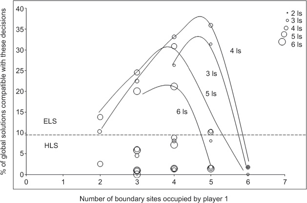
Figure 3
Possibility-Frontier Curves of local solutions (assumed to be player 1’s) as a function of the number of Is in the solution, and of the number of boundary sites that it requires. ELS and HLS=easy and hard to coordinate local solutions, respectively.
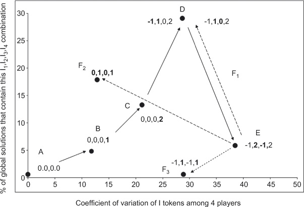
Figure 4
Pareto improvements, chicken interactions and risk of failure. The X axis is a measure of inequality in number of Is placed by each player on the board. Actual number of Is is not disclosed in the graph for the benefit of future players. At A, all players have an equal amount of I’s on the board. In B and C, player 4 has improved his score and also made coordination easier for all. To follow up with player 4, player 2 has dominated players 1 and 3 at D and E respectively. Further interactions can restore D (F1), improve the situation (F2), or worsen it (F3). Bold numbers indicate what players interacted to produce the situation.
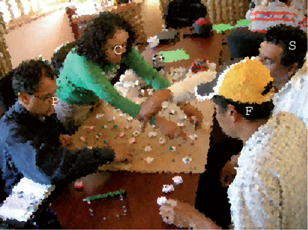
Figure 5
Players engaged in the four individual level coordination strategies. S=Suggests; C=Controls; F=Follows; P=Plays Alone. The image has been obscured for anonymity.
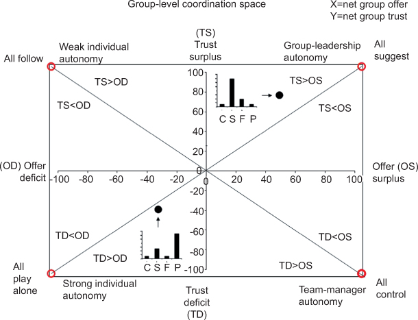
Figure 6
“Group-Level Coordination Space.” The horizontal axis is the net proportion of perceived offerers in a group: X=(C+S)–(F+P). The horizontal axis is the net proportion of perceived trusters in a group: Y=(S+F)–(C+P). Thus, the frequency distribution of S F C P reports made by a group (small histogram inside the figure) is represented by a point. See the main text for further explanation.
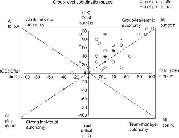
Figure 7
The position of the 40 groups in “Group Coordination Space.” Big open circles=Agroecology and rural development students (undergraduates to PhDs, but mainly MScs). Small open circles=Seasoned rural sociologists and graduate students in RPG workshop. Small filled circles=Multiactor groups (farmer leaders, government officers, NGOs, researchers) in a RPG workshop. The three subsets of players did not differ statistically in their XY position in GC space. See the main text for further explanation. Some points fall on the same x,y coordinates.