
Table 1
Models used in the time-slice simulations (30 years) for this study.
| MODELS | MODEL REFERENCE | DATA REFERENCE | COUNT OF RUNS (piClim-control, piClim-aer) |
|---|---|---|---|
| CNRM-CM6-1 | Voldoire et al. (2019) | Voldoire (2019a;b) | 1, 1 |
| CNRM-ESM2-1 | Séférian et al. (2019) | Seferian (2019a;b) | 1, 1 |
| CanESM5 | Swart et al. (2019) | Cole et al. (2019a;b) | 1, 1 |
| EC-Earth3 | Döscher et al. (2022) | EC-Earth Consortium (2020a;b) | 1, 1 |
| IPSL-CM6A-LR-INCA | Boucher et al. (2020c) | Boucher et al. (2020a;b) | 1, 1 |
| MIROC6 | Tatebe et al. (2019) | Sekiguchi and Shiogama (2019a;b) | 1, 1 |
| MPI-ESM-1-2-HAM | Mauritsen et al. (2019) | Neubauer et al. (2019a;b) | 1, 1 |
| MRI-ESM2-0 | Yukimoto et al. (2019) | Yukimoto et al. (2019a;b) | 1, 1 |
| UKESM1-0-LL | Sellar et al. (2019) | O’Connor (2019a;b) | 1, 1 |
Table 2
Models used in the transient simulations (1850–2100) for this study.
| MODELS | MODEL REFERENCE | DATA REFERENCE | COUNT OF RUNS (piClim-control, piClim-histaer) |
|---|---|---|---|
| CanESM5 | Swart et al. (2019) | Cole et al. (2019b;c) | 1, 3 |
| HadGEM3-GC31-LL | Williams et al. (2018) | Andrews (2019; 2020) | 1, 3 |
| NorESM2-LM | Seland et al. (2020) | Oliviè et al. (2019a;b) | 1, 3 |
| MIROC6 | Tatebe et al. (2019) | Sekiguchi and Shiogama (2019b;c) | 1, 3 |
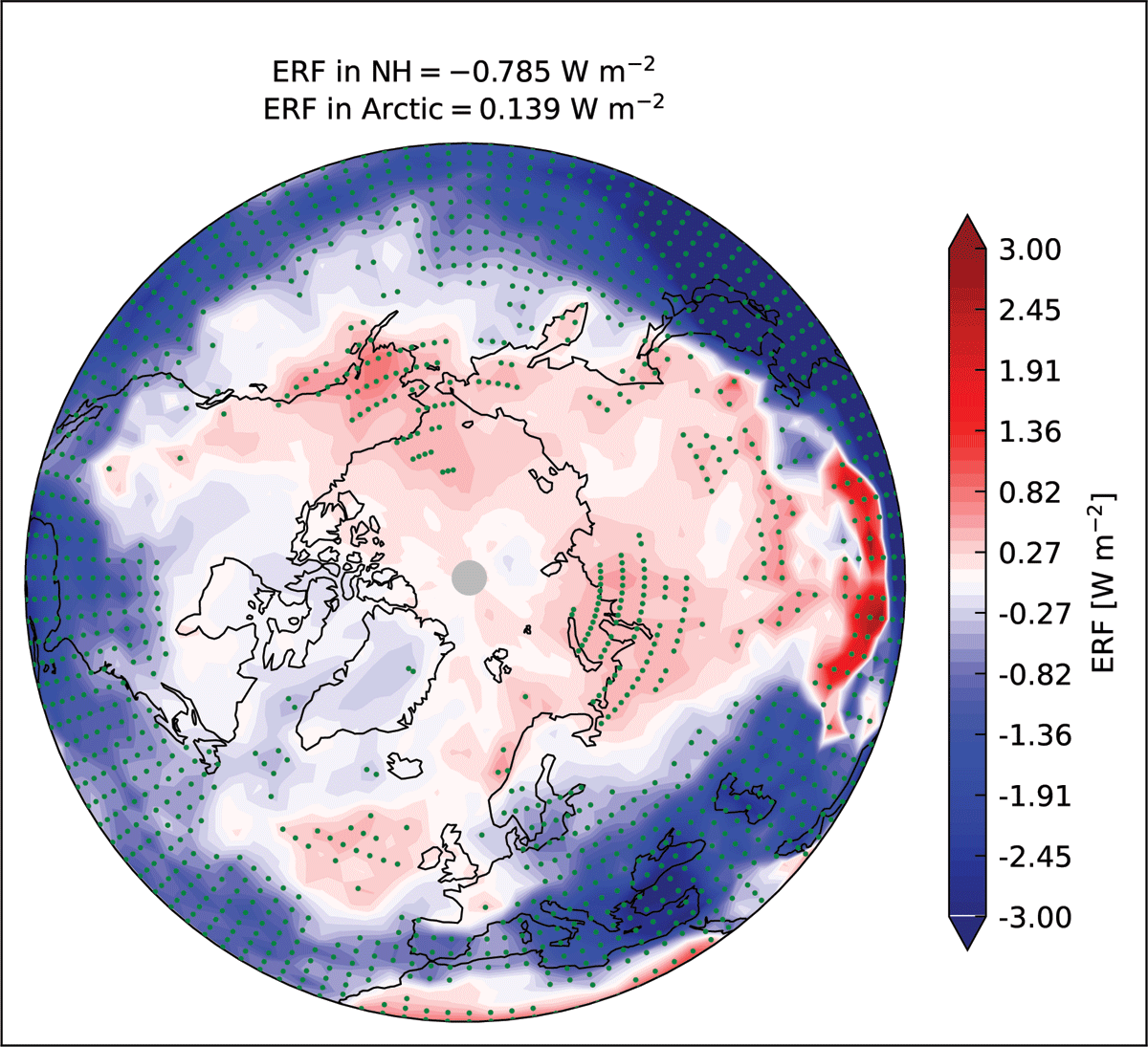
Figure 1
The present-day (2014) (W m–2) in piClim-aer during the winter season (DJF) compared to the pre-industrial condition in piClim-control (1850) for the NH between 20°N and 90°N. The green dots refer to the statistical significance at a 75% confidence level, as determined by a t-test. The piClim-aer simulation is configured with present-day aerosols and fixed-SST, and piClim-control maintains forcing components at pre-industrial levels (1850). The figure shows the multi-model average of the nine models listed in Table 1.
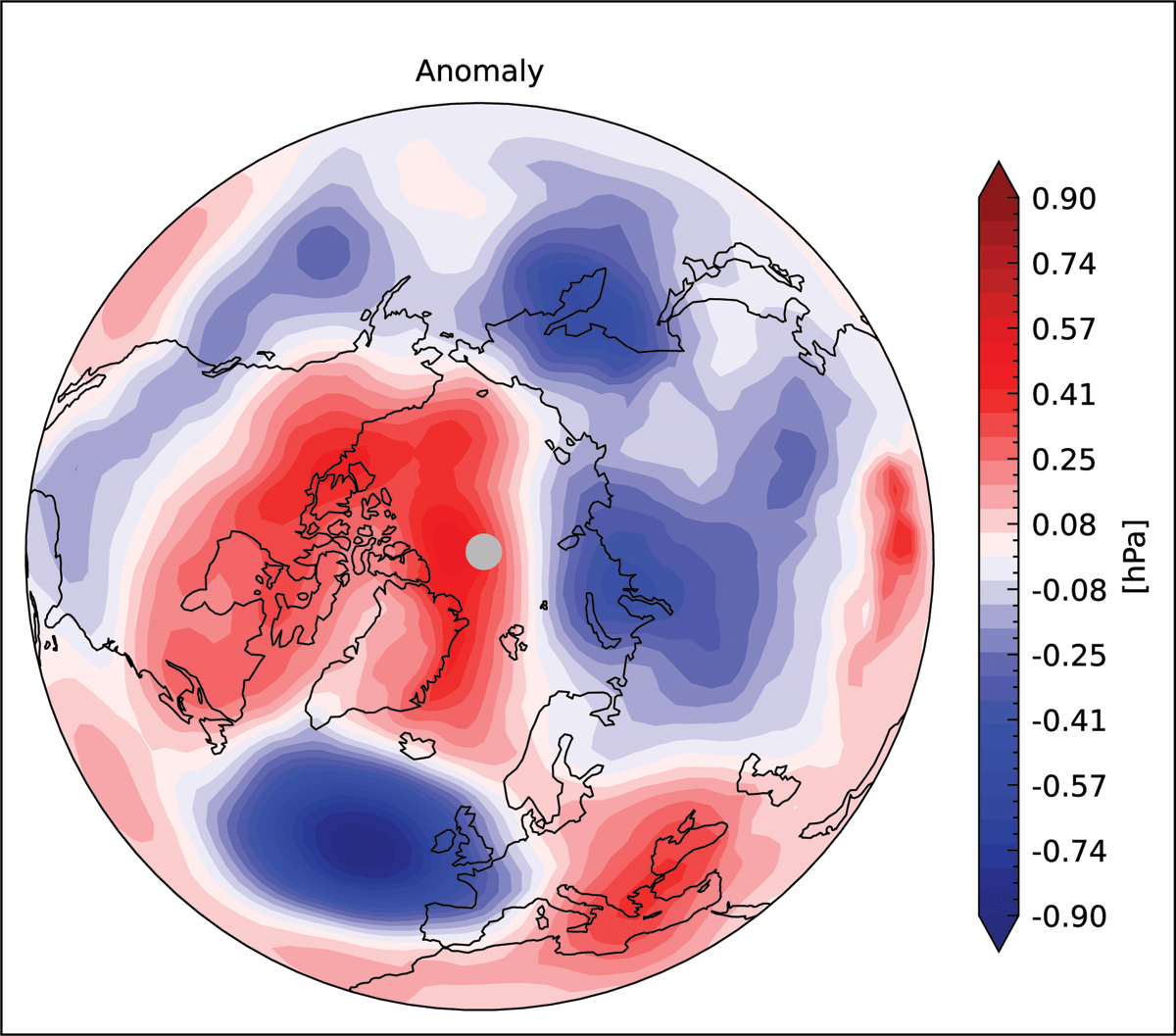
Figure 2
Leading empirical orthogonal functions (EOF) of the winter (DJF) mean SLP (hPa) anomalies for piClim-aer (2014) compared to the pre-industrial condition in piClim-control (1850) for the NH between 20°N and 90°N. The piClim-aer simulation is configured with present-day aerosols and fixed-SST, and piClim-control maintains forcing components at pre-industrial levels (1850).
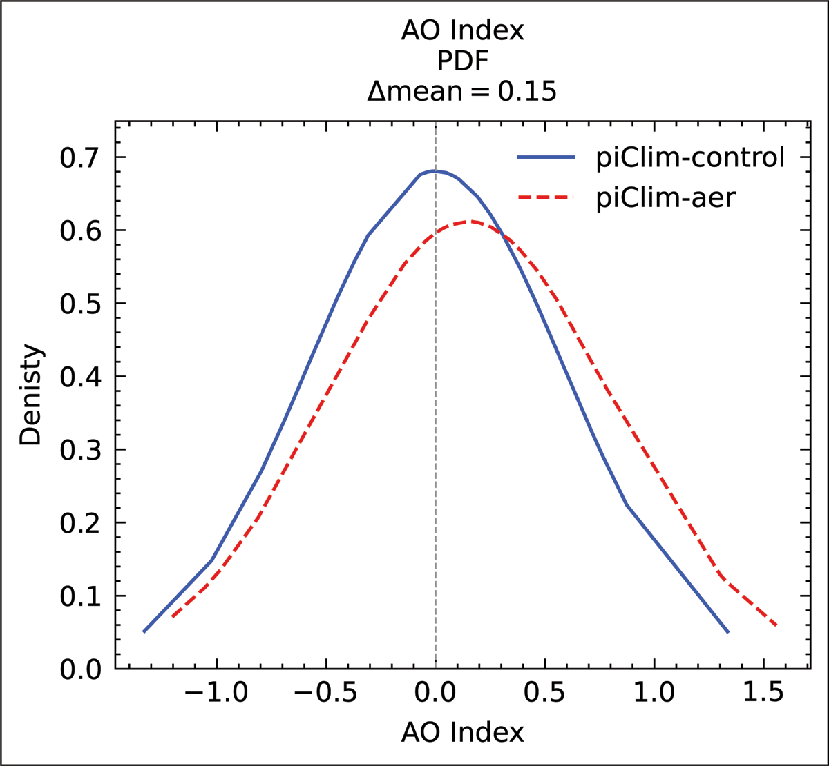
Figure 3
Comparison of probability density function (PDF) of AOI for the piClim-control and piClim-aer during the winter (DJF). Both simulations cover a 30-year period. In piClim-aer, present-day (2014) aerosols are applied with fixed-SST, whereas piClim-control maintains all forcing components at pre-industrial levels (1850). By each simulation, the multi-model mean SLP is first calculated, and the AOI and its corresponding PDF are derived from this multi-model mean SLP.
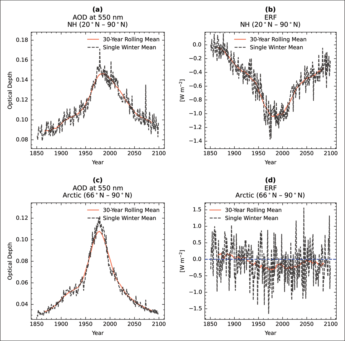
Figure 4
Time series of (a, b) aerosol optical depth at 550 nm and (c, d) (W m–2) during winter (DJF) from the piClim-histaer transient simulation (1851–2099), shown for the NH between 20°N and 90°N (a, c), and the Arctic region between 66°N and 90°N (b, d). The dashed black lines are for single winter means, the red solid lines refer to the 30-year moving average of winter means, and the blue dashed line indicates the zero value. The both figures show the multi-model average of the four models listed in Table 2.
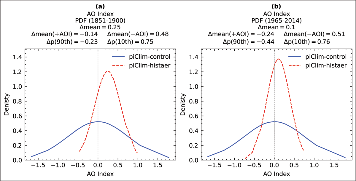
Figure 5
Comparison of PDF of AOI for the piClim-control and piClim-histaer during the winter (DJF). PDF for (a) low aerosol loading scenario (1851–1900) and (b) high aerosol burden (1965–2014), respectively. refers to the anomaly of the average AOI in piClim-histaer’s period from the average piClim-control. and refer to the anomalies of the average positive and negative index values respectively.
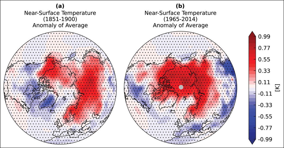
Figure 6
Comparison of SAT (K) anomaly relative to piClim-control during the winter (DJF) for (a) low aerosol loading scenario (1851–1900) and (b) high aerosol burden (1965–2014), respectively. The black dots indicate the statistical significance at a 75% confidence level.
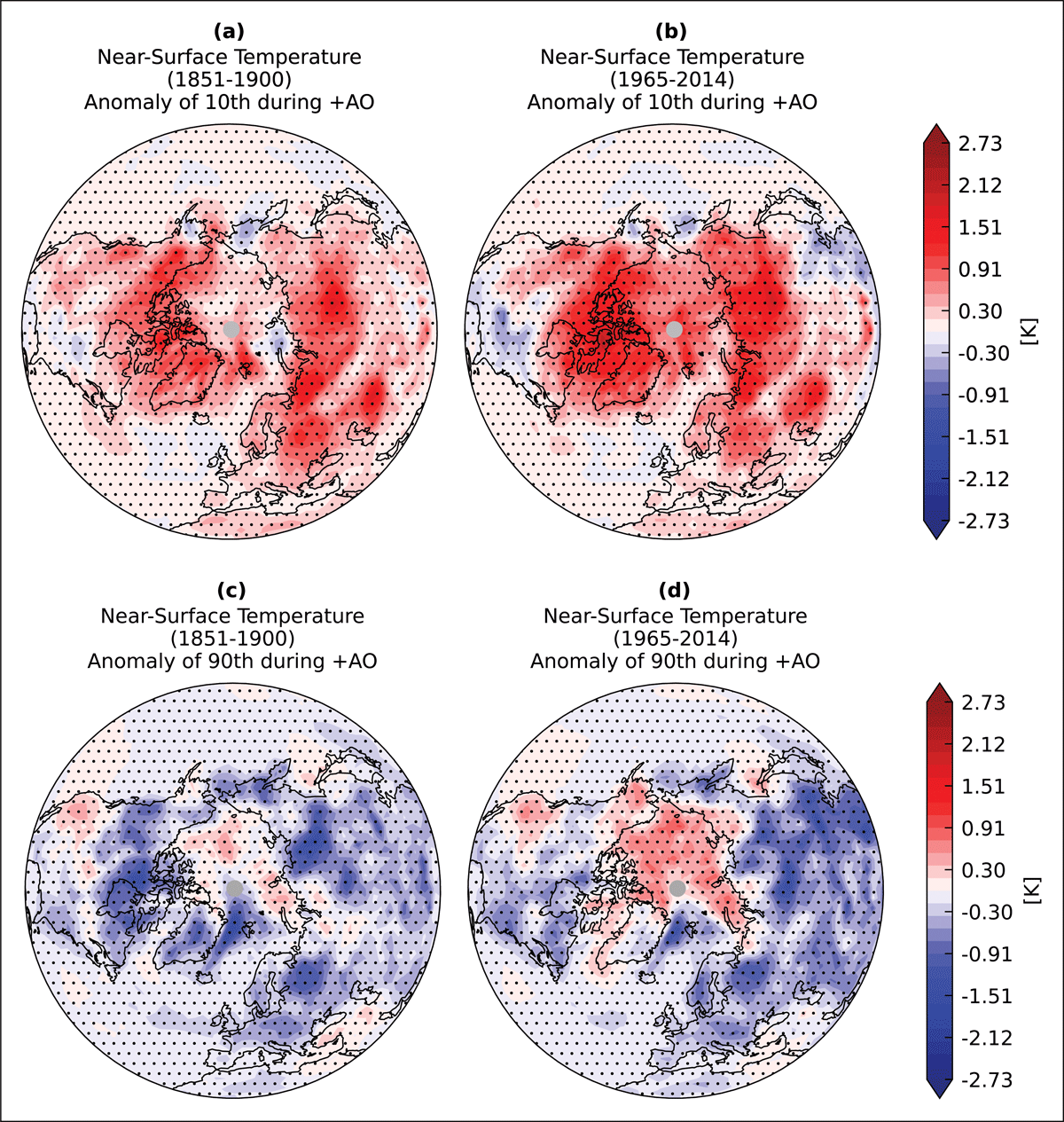
Figure 7
Comparison of 10th and 90th percentiles of SAT (K) anomaly relative to piClim-control during the winter (DJF) for positive AO phase. Panels (a) and (b) show the 10th percentile of SAT anomaly for low aerosol loading scenario (1851–1900) and high aerosol scenario (1965–2014), respectively. Panels (c) and (d) show the 90th percentile of SAT anomalies for the same two scenarios. The black dots indicate the statistical significance at a 75% confidence level.
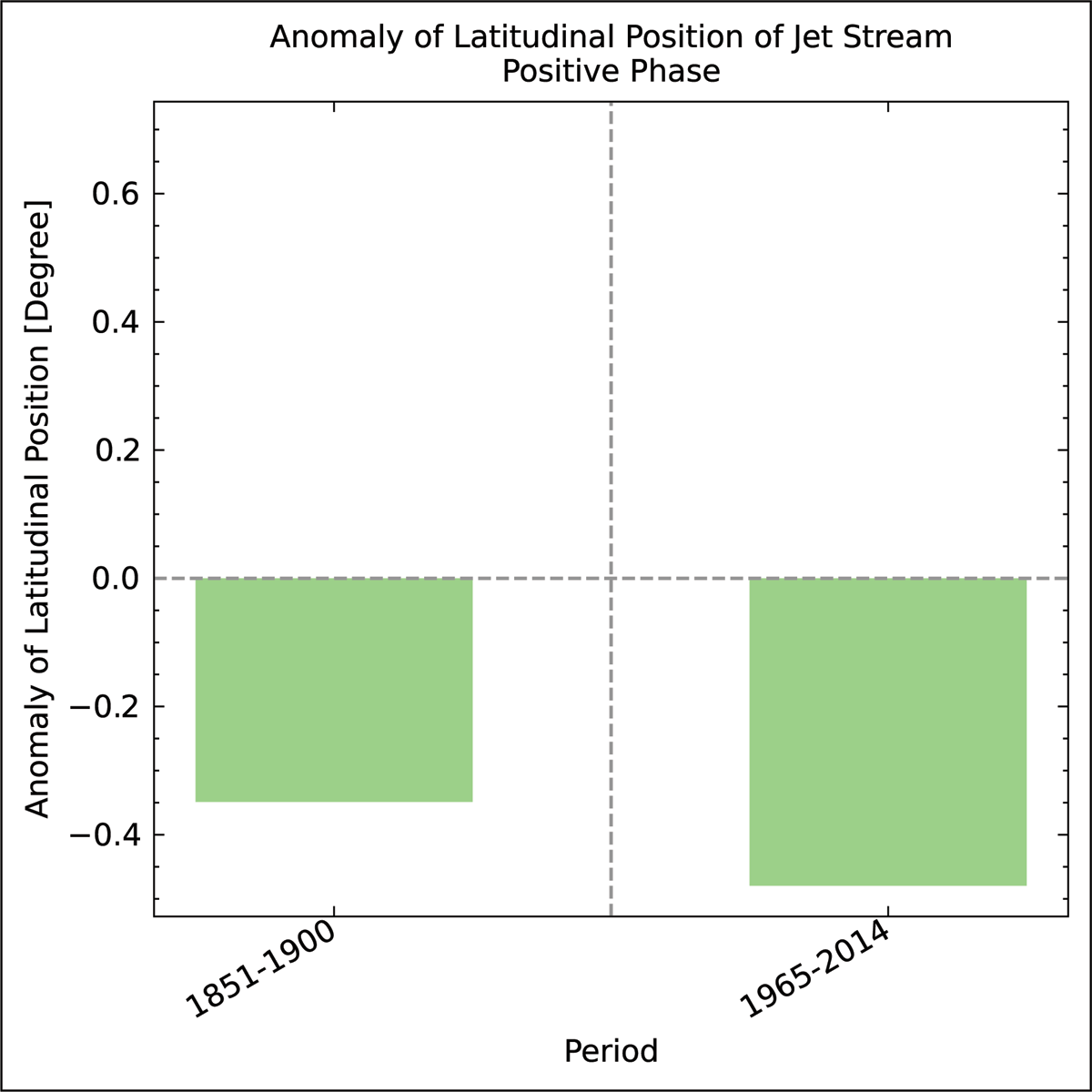
Figure 8
Anomalies of the latitudinal position of the jet stream in piClim-histaer during the positive AO with respect to piClim-control. The periods 1851–1900 and 1965–2014 represent low and high aerosol loading scenarios, respectively.
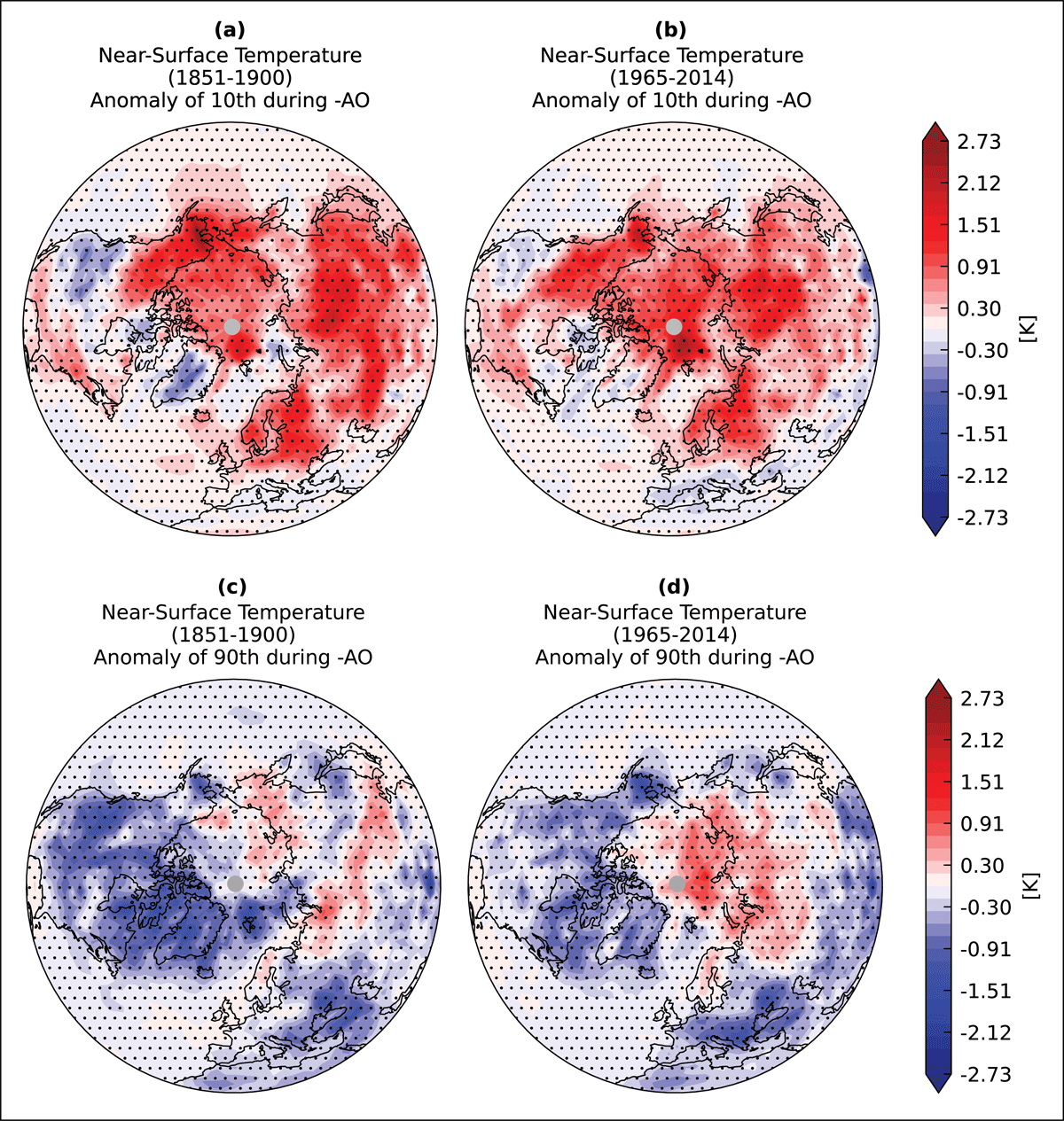
Figure 9
Comparison of 10th and 90th percentiles of SAT (K) anomaly relative to piClim-control during the winter (DJF) for negative AO phase. Panels (a) and (b) show the 10th percentile of SAT anomaly for low aerosol loading scenario (1851–1900) and high aerosol scenario (1965–2014), respectively. Panels (c) and (d) show the 90th percentile of SAT anomalies for the same two scenarios. The black dots indicate the statistical significance at a 75% confidence level.
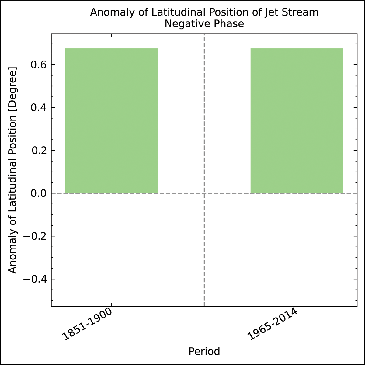
Figure 10
Anomalies of the latitudinal position of the jet stream in piClim-histaer during the negative AO with respect to piClim-control. The periods 1851–1900 and 1965–2014 represent low and high aerosol loading scenarios, respectively.
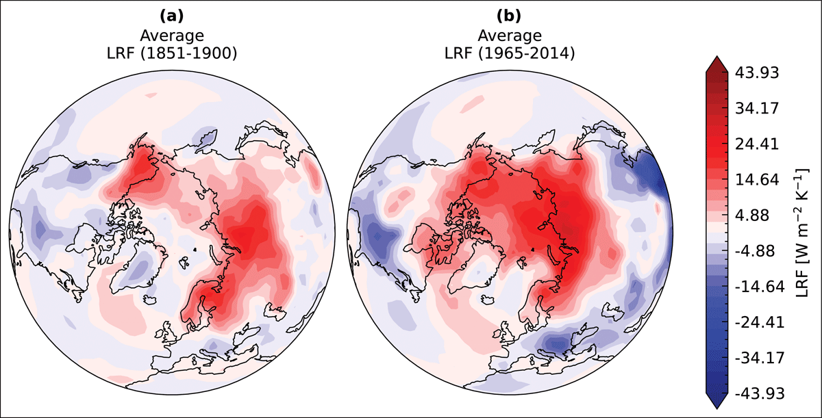
Figure 11
Comparison of the LRF (W m–2 K–1) in the NH (between 20°N and 90°N) during (a) low aerosol loading scenario (1851–1900) and (b) high aerosol scenario (1965–2014) for the winter (DJF).
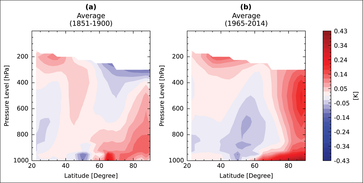
Figure 12
The latitudinal cross-section of the winter (DJF) temperature anomalies (K) relative to piClim-control in the NH (between 20°N and 90°N) during (a) low aerosol loading scenario (1851–1900) and (b) high aerosol scenario (1965–2014).
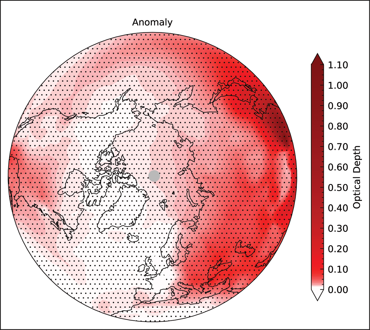
Figure A.1
Aerosol optical depth (AOD) anomalies in piClim-aer from piClim-control over the NH between 20°N and 90°N during the winter (DJF). The black dots indicate where the AOD difference between piClim-control and piClim-aer is statistically significant at a 75% confidence level.
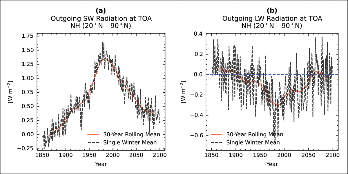
Figure A.2
Time series of anomalies of (a) outgoing SW radiation at TOA and (b) outgoing LW radiation at TOA (in W m–2) in piClim-histaer from piClim-control for winter (DJF). The dashed black lines are for single winter means, and the red solid lines refer to the 30-year moving average of winter means, and the blue dashed line indicates the zero value. The values are for the NH between 20°N and 90°N from 1851 to 2099.
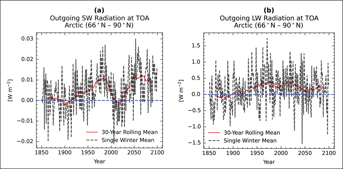
Figure A.3
Time series of anomalies of (a) outgoing SW radiation at TOA and (b) outgoing LW radiation at TOA (in W m–2) in piClim-histaer from piClim-control for winter (DJF). The dashed black lines are for single winter means, the red solid lines refer to the 30-year moving average of winter means, and the blue dashed line indicates the zero value. The values are for the Arctic between 66°N and 90°N from 1851 to 2099.
Table A.1
and its solar and terrestrial components over the NH domain between 20°N and 90°N as derived from the time-slice simulations (piClim-aer) relative to the reference simulations (piClim-control). Units are in W m–2.
| MODELS | ERFaer | CHANGE OF UPWARD SW RADIATION AT TOA | CHANGE OF UPWARD LW RADIATION AT TOA |
|---|---|---|---|
| CNRM-CM6-1 | –1.168 | 1.255 | –0.09 |
| CNRM-ESM2-1 | –0.502 | 0.89 | –0.391 |
| CanESM5 | –0.432 | 0.441 | –0.008 |
| EC-Earth3 | –0.398 | 0.55 | –0.15 |
| IPSL-CM6A-LR-INCA | –0.562 | 0.498 | 0.058 |
| MIROC6 | –0.715 | 1.104 | –0.394 |
| MPI-ESM-1-2-HAM | –1.358 | 1.496 | –0.135 |
| MRI-ESM2-0 | –1.055 | 1.915 | –0.857 |
| UKESM1-0-LL | –0.753 | 0.929 | –0.176 |
| Multi-Model Average | –0.785 | 1.024 | –0.24 |
Table A.2
and its solar and terrestrial components over the Arctic between 66°N and 90°N as derived from the time-slice simulations (piClim-aer) relative to the reference simulations (piClim-control). Units are in W m–2.
| MODELS | ERFaer | CHANGE OF UPWARD SW RADIATION AT TOA | CHANGE OF UPWARD LW RADIATION AT TOA |
|---|---|---|---|
| CNRM-CM6-1 | 0.07 | 0.015 | –0.084 |
| CNRM-ESM2-1 | 0.593 | –0.005 | –0.588 |
| CanESM5 | 0.046 | –0.057 | 0.011 |
| EC-Earth3 | 0.695 | 0.004 | –0.697 |
| IPSL-CM6A-LR-INCA | 1.148 | 0.027 | –1.177 |
| MIROC6 | 0.422 | 0.012 | –0.435 |
| MPI-ESM-1-2-HAM | –0.078 | –0.026 | 0.106 |
| MRI-ESM2-0 | –0.806 | 0.002 | 0.806 |
| UKESM1-0-LL | –0.863 | –0.007 | 0.87 |
| Multi-Model Average | 0.139 | –0.004 | –0.134 |
Table A.3
and its solar and terrestrial components over the NH domain outside the Arctic (i.e., between 20°N and 66°N) as derived from the time-slice simulations (piClim-aer) relative to the reference simulations (piClim-control). Units are in W m–2.
| MODELS | CHANGE OF UPWARD SW RADIATION AT TOA | CHANGE OF UPWARD LW RADIATION AT TOA | |
|---|---|---|---|
| CNRM-CM6-1 | –1.356 | 1.444 | –0.091 |
| CNRM-ESM2-1 | –0.669 | 1.026 | –0.361 |
| CanESM5 | –0.497 | 0.508 | –0.011 |
| EC-Earth3 | –0.566 | 0.634 | –0.066 |
| IPSL-CM6A-LR-INCA | –0.805 | 0.565 | 0.233 |
| MIROC6 | –0.887 | 1.27 | –0.388 |
| MPI-ESM-1-2-HAM | –1.568 | 1.746 | –0.175 |
| MRI-ESM2-0 | –1.093 | 2.201 | –1.106 |
| UKESM1-0-LL | –0.737 | 1.067 | –0.331 |
| Multi-Model Average | –0.911 | 1.164 | –0.255 |