
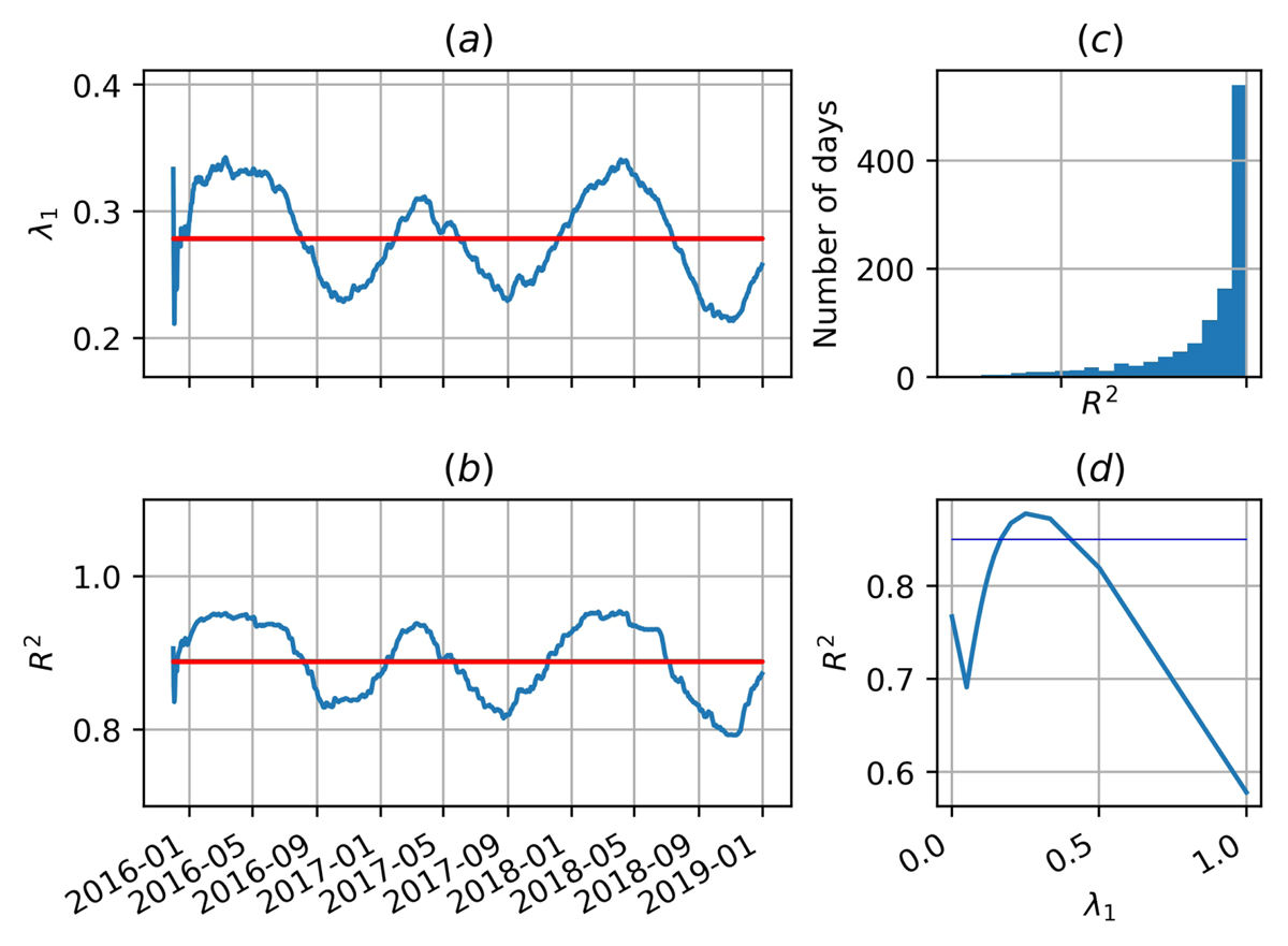
Figure 1
Determination of optimal values of λ1 over the whole period: (a) is the time series of optimal λ1 values (in blue) and its mean value (in red), (b) is the associated correlation factor, with daily values (in blue) and its mean value (in red), (c) is the distribution of the correlation factor over the whole period and (d) are the mean correlation factors over the whole period for each λ1 value.
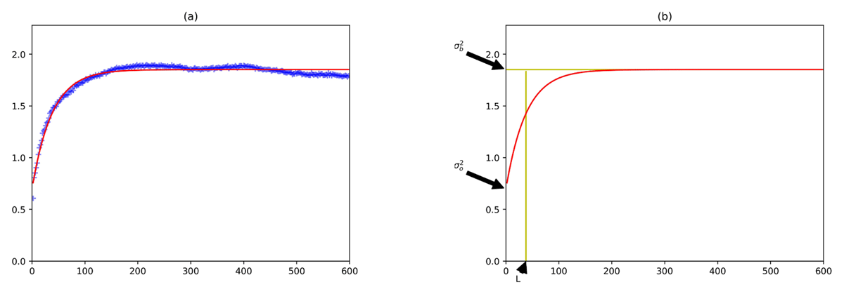
Figure 2
Experimental (blue cross) and theoretical (red line) semi-variograms (a) and determination of , and L (b).
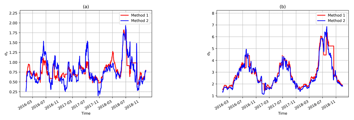
Figure 3
Daily values of (a) and (b) for the two methods.
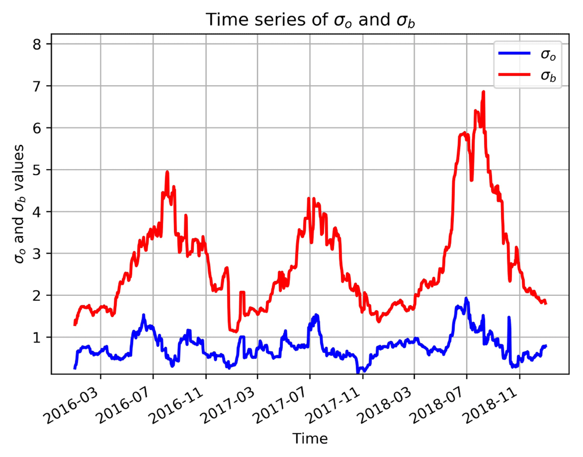
Figure 4
Daily values of and for the Box-Cox transformation with .
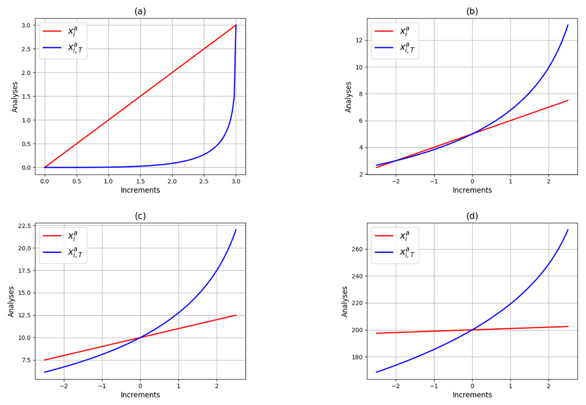
Figure 5
Put on evidence of the bias induced by the Box-Cox transformation. The red line stands for the analysis wanted () and the blue line stands for the analysis obtained after the Box-Cox transformation () for background values fixed at 0 mm (a), 5 mm (b), 10 mm (c) and 200 mm (d).
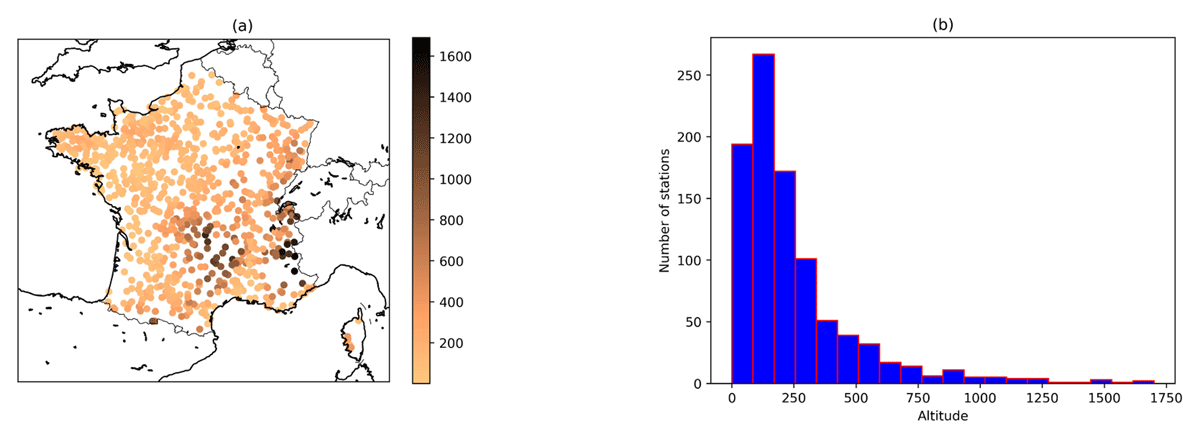
Figure 6
Spatial coverage of the evaluation observations’ altitudes (m) (a) and number of stations per altitude (b).
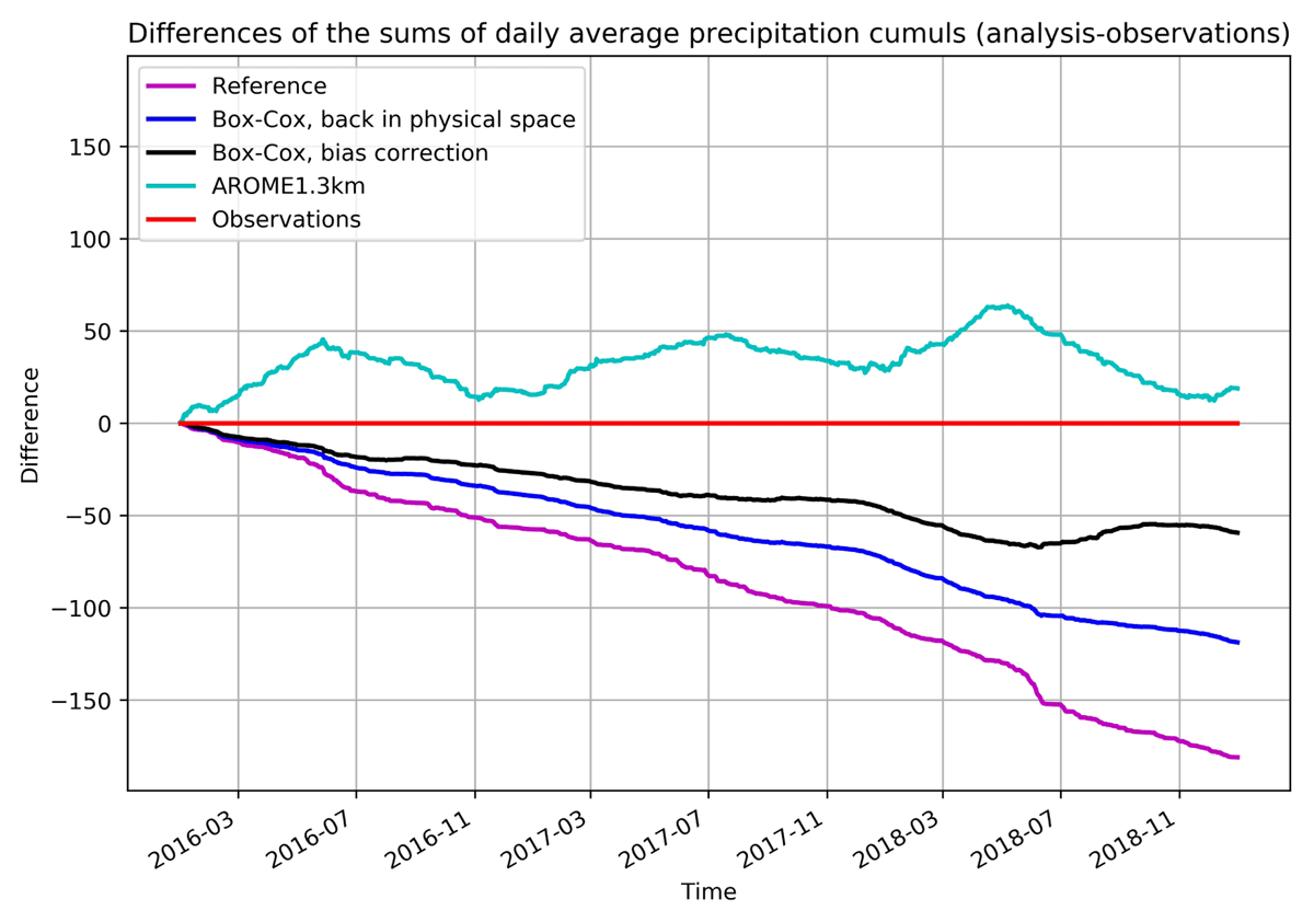
Figure 7
Differences of the accumulated daily precipitation averaged over France between the observations and the different experiments.
Table 1
Values of the scores for the different experiments.
| EXPERIMENT | BIAS (mm) | RMSE (mm) | DIFFERENCE AT THE END OF THE PERIOD | |
|---|---|---|---|---|
| AROME1-3 km | 1.73 10–2 | 3.85 | +18.91 mm (+0.71%) | |
| Reference | –0.17 | 2.54 | –180.91 mm (–6.84%) | |
| Box-Cox | Back in physical space | –0.11 | 2.38 | –118.63 mm (–4.48%) |
| Correction (Eq.(21)) | –5.41 10–2 | 2.40 | –59.24 mm (–2.24%) | |
| Correction (Eq. (24)) | –5.67 10–2 | 2.39 | –62.14 mm (–2.35%) | |
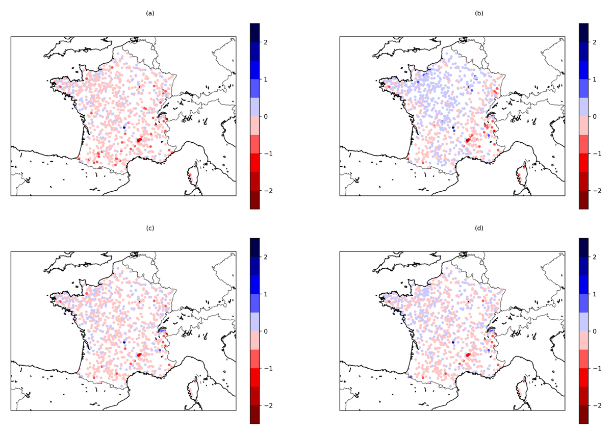
Figure 8
Bias over the whole period for the reference (a), the background (b), the Box-Cox experiment with a simple back in physical space (c) and after bias correction (d). Blue points mean an overestimation while red ones mean an underestimation.
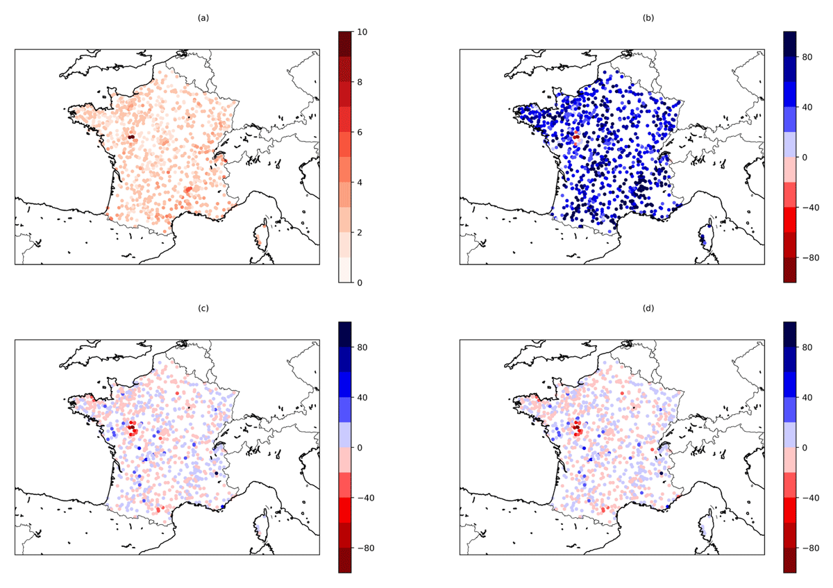
Figure 9
RMSE over the whole period for the reference (a) and percent of improvement for the background (b), the Box-Cox experiment with a simple back in physical space (c) and after bias correction (d). Blue points mean worse RMSE while red ones mean better ones.
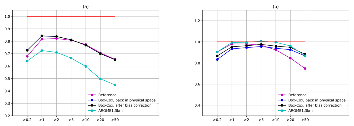
Figure 10
HSS (a) and FBI (b) for the different experiments.
Table 2
Number of dry days for the observations, the experiments and their correlation R.
| EXPERIMENT | DRY DAYS | R | |
|---|---|---|---|
| Observations | 491 155 | 1.00 | |
| AROME-1.3 km | 416 145 | 0.64 | |
| Reference | 386 309 | 0.60 | |
| Box-Cox | Back in physical space | 445 145 | 0.66 |
| Correction | 373 206 | 0.66 | |
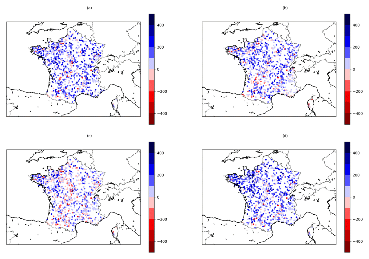
Figure 11
Difference of the number of dry days between observations and the analyses during the whole period for the reference (a), the background (b), the Box-Cox experiment with a simple back in physical space (c) and after bias correction (d). Blue (resp. red) points represent an underestimation (resp. overestimation) of the number of dry days.
Table 3
Seasonal bias for the different experiments (mm).
| EXPERIMENT | DJF | MAM | JJA | SON | |
|---|---|---|---|---|---|
| AROME1-3 km | 0.17 | 0.19 | –0.15 | –0.14 | |
| Reference | –0.14 | –0.19 | –0.21 | –0.12 | |
| Box-Cox | Back in physical space | –0.13 | –0.13 | –9.97 10–2 | –7.15 10–2 |
| Correction | –0.11 | –9.20 10–2 | 8.62 10–2 | –2.44 10–2 | |
Table 4
Seasonal RMSE for the different experiments (mm).
| EXPERIMENT | DJF | MAM | JJA | SON | |
|---|---|---|---|---|---|
| AROME1-3 km | 3.18 | 3.95 | 4.37 | 3.79 | |
| Reference | 2.06 | 2.81 | 2.93 | 2.24 | |
| Box-Cox | Back in physical space | 1.94 | 2.43 | 2.88 | 2.15 |
| Correction | 1.94 | 2.43 | 2.91 | 2.16 | |
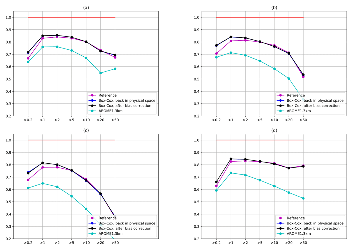
Figure 12
HSS for the different experiments during winter (a), spring (b), summer (c) and autumn (d).
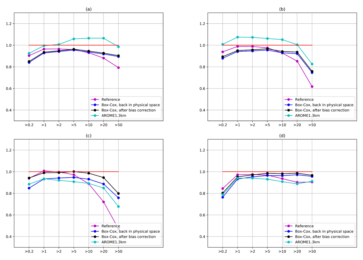
Figure 13
FBI for the different experiments during winter (a), spring (b), summer (c) and autumn (d).
Table 5
Number of seasonal dry days for the observations, the experiments and their correlation R.
| EXPERIMENT | DJF | MAM | JJA | SON | |||||
|---|---|---|---|---|---|---|---|---|---|
| Dry days | R | Dry days | R | Dry days | R | Dry days | R | ||
| Observations | 92855 | 1.00 | 120889 | 1.00 | 156684 | 1.00 | 120727 | 1.00 | |
| AROME-1.3 km | 66946 | 0.64 | 95485 | 0.61 | 143439 | 0.69 | 110275 | 0.55 | |
| Reference | 69617 | 0.60 | 96545 | 0.54 | 127395 | 0.64 | 92752 | 0.51 | |
| Box-Cox | Back in phys.space | 80973 | 0.70 | 109431 | 0.61 | 144184 | 0.69 | 110557 | 0.59 |
| Correction | 73000 | 0.70 | 98434 | 0.60 | 113290 | 0.67 | 88482 | 0.59 | |
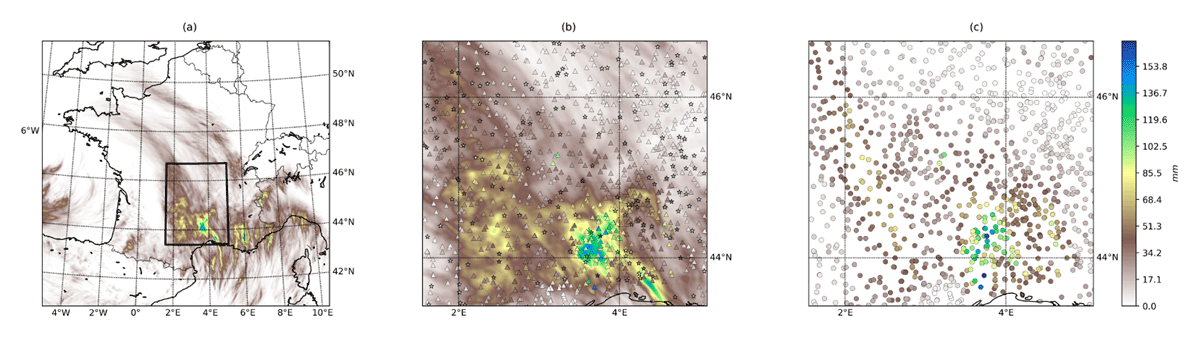
Figure 14
Convective event of the 16/09/2016 modelled by AROME-1.3 km over the whole domain (a) and over the study area (b). Stars corresponds to evaluation observations and triangles for observations used as input of the MESCAN analysis. All the available observations over the study area (c).
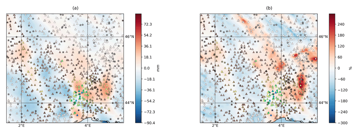
Figure 15
Difference of the reference precipitation analysis and the background AROME-1.3 km during the convective event of the 16/09/2016 over the study area (a) and percent of added precipitation of the reference compared to the background AROME-1.3 km over the study area (b).
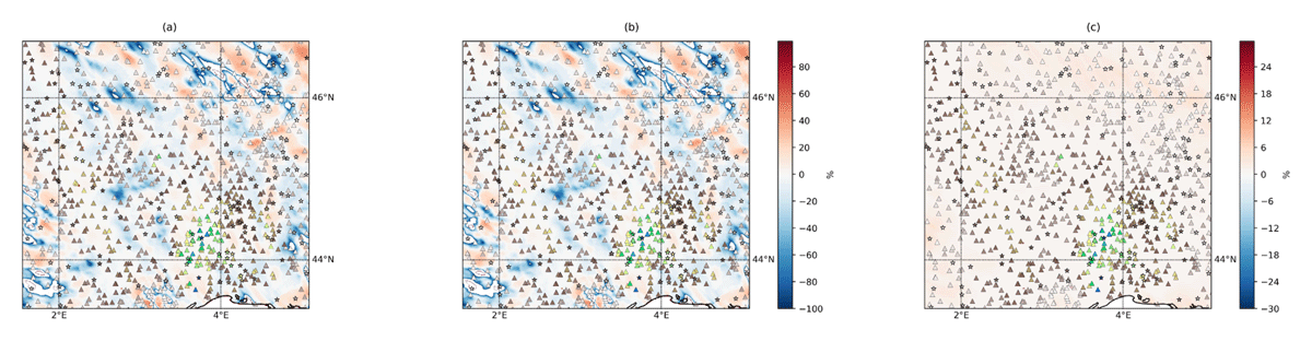
Figure 16
Percent of added precipitation of the transformed back into physical space analysis (a) and analysis after bias correction (b) compared to the reference and percent of added precipitation of the analysis after bias correction compared to the transformed back into physical space analysis (c).
Table 6
Bias and RMSE values for the different experiments on 16/09/2016 over the whole domain and over the study area (between parenthesis).
| EXPERIMENT | BIAS (mm) | RMSE (mm) | |
|---|---|---|---|
| AROME-1.3 km | –0.08 (–1.61) | 13.71 (20.61) | |
| Reference | –0.91 (–3.32) | 7.49 (13.85) | |
| Box-Cox | Back in physical space | –0.55 (–2.36) | 7.56 (14.09) |
| Correction (Eq. (21)) | –0.41 (–2.18) | 7.56 (14.05) | |
| OBSERVATIONS | |||
|---|---|---|---|
| Yes | No | ||
| Model | Yes | a | b |
| No | c | d | |