
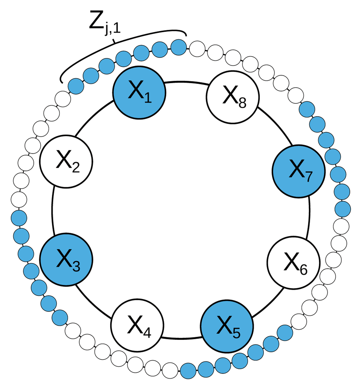
Figure 1
A recreation of a similar image by Wilks (2005), that illustrates the two timescale Lorenz-96 model.
Table 1
Summary of Lyapunov Exponents.
| Largest Lyapunov exponent λ1 | 2.3098 |
| Error doubling time | 0.3 time units |
| Number of strictly positive Lyapunov exponents | 14 |
| Number of neutral, λ ∈ [–1E –2, 1E –2], exponents | 1 |
| Number of strictly negative Lyapunov exponents | 26 |
| Kaplan-Yorke dimension | 29.4694 |
| Kolmogorov-entropy | 14.8409 |
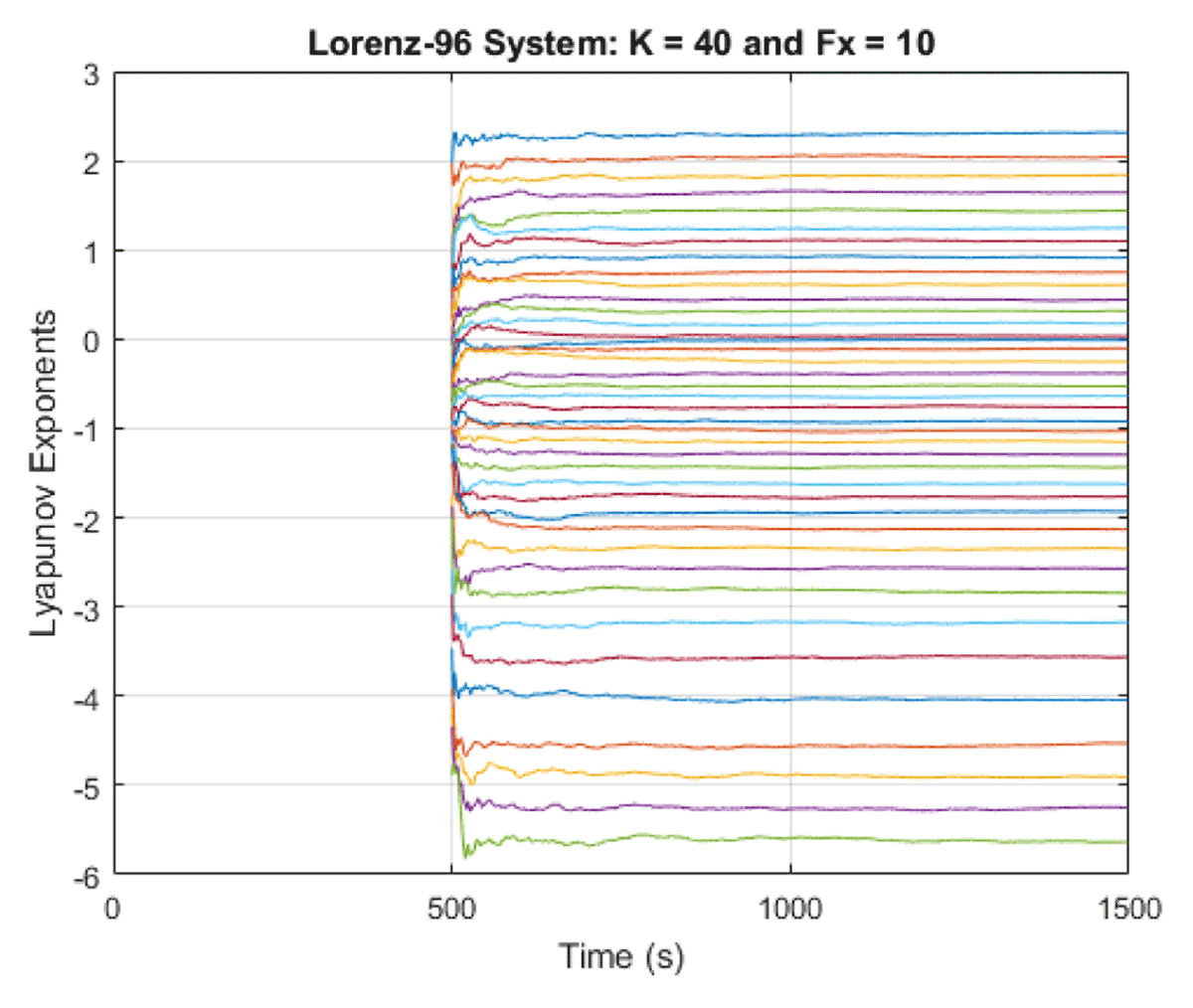
Figure 2
Time evolution of Lyapunov exponents for the Lorenz-96 system.
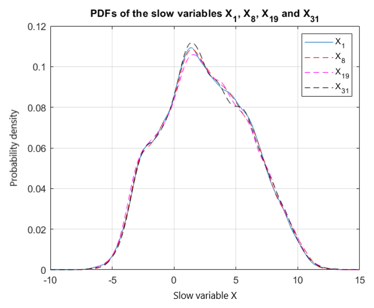
Figure 3
PDFs of the slow variables X1, X8, X19 and X31.
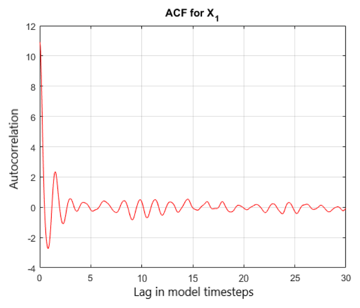
Figure 4
ACF of the slow variable X1.
Table 2
Evaluation of each method.
| METHOD | MSPE | AVERAGE K-L DIVERGENCE |
|---|---|---|
| Regression | 0.03606 | 0.06729 |
| Compressed sensing (Raw) | 5.9993 | 1.9891 |
| Compressed sensing [1] (Setting biases to zero) | 0.03398 | 0.10099 |
| Compressed sensing [2] (Setting biases to average bias) | 0.03440 | 0.07351 |
| Compressed sensing [3] (Adding noise to average bias) | 0.03387 | 0.05919 |
Table 3
AR evaluation of residuals.
| METHOD | φ | σ | σe | MSPE | AVE. K-L DIVERGENCE |
|---|---|---|---|---|---|
| Regression | 0.9453 | 0.2265 | 0.6945 | 0.02624 | 0.07692 |
| Compressed sensing | 0.9981 | 0.1710 | 2.775 | 0.02066 | 0.07142 |
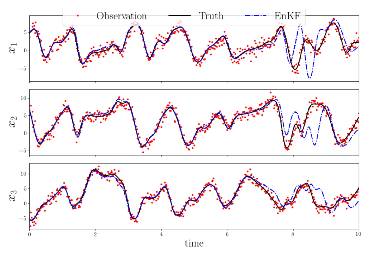
Figure 5
True trajectories, observations and EnKF with Wilks’ parametrized model.
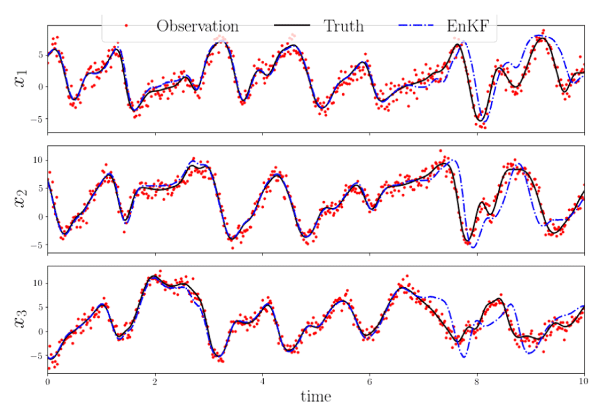
Figure 6
True trajectories, observations and EnKF with compressed sensing model.
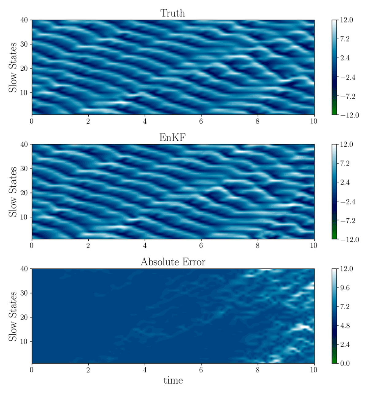
Figure 7
Depiction of Lorenz-96 true and EnKF prediction trajectories for 40 components (Auto-regressive Wilks’ parameterization).
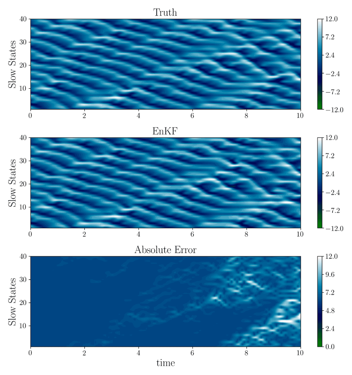
Figure 8
Depiction of Lorenz-96 true and EnKF prediction trajectories for 40 components (Auto-regressive compressed sensing).