
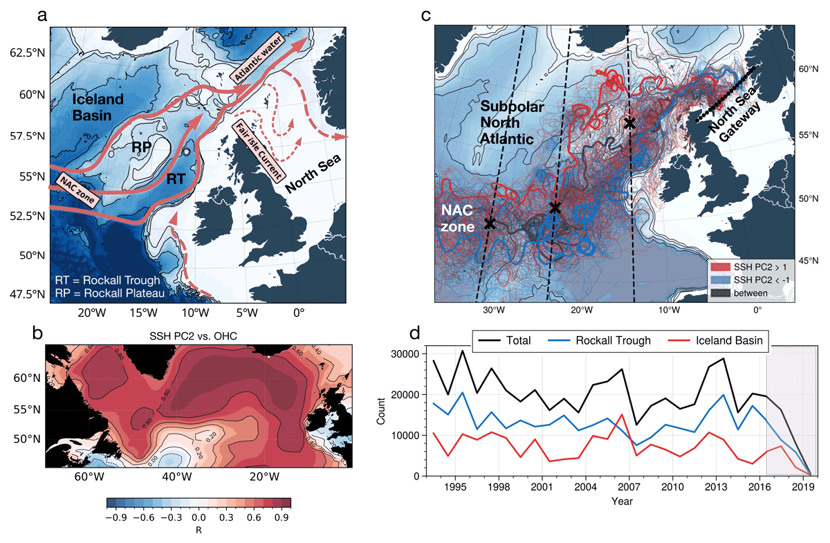
Figure 1
(a) Schematic of Atlantic Water pathways in the eastern SPNA toward the North Sea gateway (circles in panel c). (b) Spatial correlation between annually averaged SSH PC2 (1993–2019) and ocean heat content (OHC; 0–700 m) variability from the EN4 dataset (Good et al., 2013). OHC has been deseasonalized and detrended before the analysis. (c) Spaghetti plot of backward trajectories initialized at the North Sea gateway and backtracked to the NAC zone (panel a). Thin solid trajectories show multiple examples of particle pathways under varying SPNA conditions indicated by SSH PC2 phases: warm (SSH PC2 > 1; red), cold (SSH PC2 < –1; blue), and neutral (–1 < SSH PC2 < 1; gray). Thick solid lines represent one representative trajectory for each SSH PC2 phase, illustrating the full path from the NAC zone to the North Sea gateway. Dashed meridional sections with crosses indicate locations used for diagnosing Lagrangian transport in Figure 4. (d) Annual mean particle count reaching the easternmost meridional section at 14°W (black line). The thick black cross at 58°N (panel c) marks the approximate boundary separating particles originating from the Iceland Basin (red line) and the Rockall Trough (blue line). The drop in particle count during the final years of the time series is due to an edge effect, as trajectories require sufficient time to reach the meridional sections. This period is highlighted with a gray box.
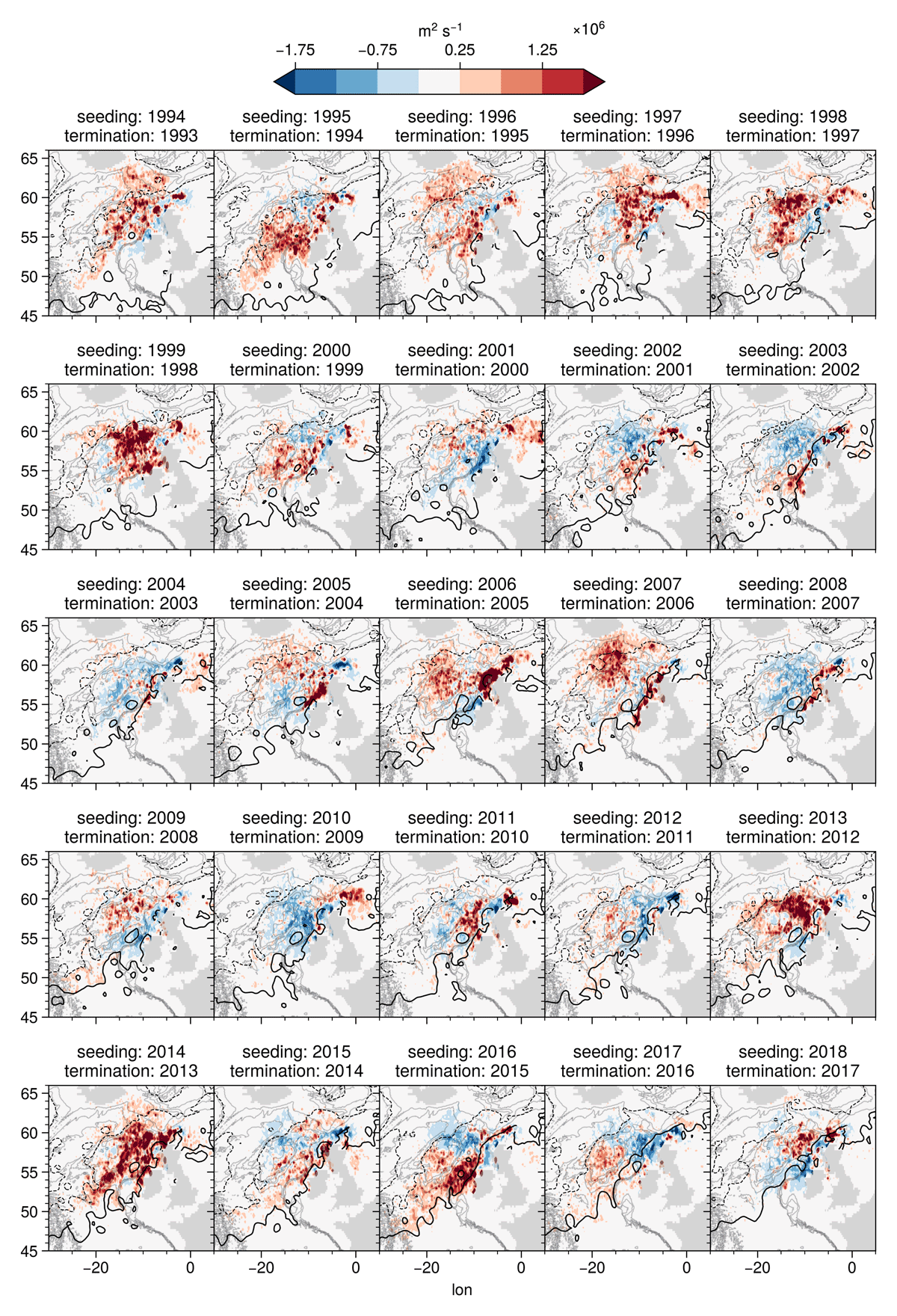
Figure 2
Anomalies of annual parcel transport 12 months before seeding overlaid with ADT contours at –0.4,–0.2, 0, 0.2, and 0.4 m. ADT is averaged using a 2-year pyramid-shaped weighting scheme. Annually, the total transport varies from 68% (seeding 2010, termination 2009) of the long-term mean up to 147% (seeding 2014, termination 2013). This results in years with same sign anomalies throughout. Percentages refer to the total transport relative to the time mean, for example, 68%/147% indicates a year with 32%/47% less/more transport than the time mean.
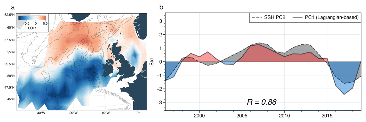
Figure 3
(a) The first leading mode of variability (EOF1) based on the Lagrangian trajectories. The analysis is performed on the anomalies of annual parcel transports 12 months before seeding. (b) Three-year rolling average of the first principal component of the Lagrangian trajectories (solid line with red-blue shading) overlaid with SSH PC2 (dashed line with gray shading). The correlation coefficient between the two time series is 0.86.
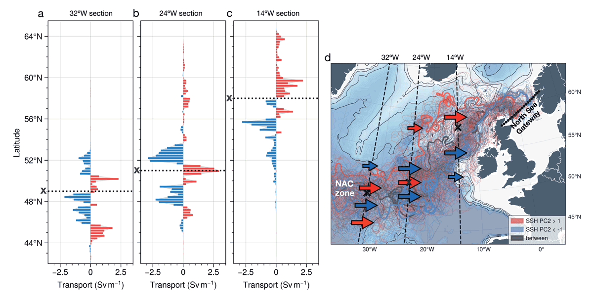
Figure 4
(a) Composite difference of Lagrangian transport at the easternmost meridional section, calculated as the difference between periods of anomalously positive SSH PC2 (>1 std) and anomalously negative SSH PC2 (<–1 std). (b–c) Same as (a), but for the central and westernmost meridional sections, respectively. Dashed lines and crosses on the y-axes indicate the approximate central position of the main flow (see panel d). (d) Schematic representation of transport anomalies, shown as arrows, at the three longitudinal sections (panels a–c) associated with contrasting SPNA periods, as indicated by SSH PC2 phases. These anomalies are overlaid on the trajectory pathways from Figure 1c. The positions of the crosses correspond to those indicated on the y-axes in panels (a–c).