
1 Introduction
High-impact weather phenomena are often triggered by convective-scale disturbances embedded in a synoptic-scale circulation. For example, mesoscale convective systems can develop in synoptic-scale moisture tongue structures such as the Meiyu–Baiu frontal zone or deep convective clouds in a tropical cyclone. To numerically simulate the small-scale structures in these hierarchical phenomena, we require a forecast model with fine horizontal resolution (1–4 km) (Kanada and Wada, 2016; Fukui and Murata, 2021). Although state-of-the-art high-performance supercomputer systems are capable of such high-resolution simulations in the global domain, a sufficient resolution is efficiently realized by a nested system embedding a high-resolution limited-area model (LAM) in a relatively coarse-resolution global model (GM).
The prediction skills of GMs in large-scale circulations have been improved by increasingly available satellite observations and active developments of numerical models and data assimilation (DA) at operational numerical weather prediction (NWP) centers. By contrast, LAM analysis systems cannot properly represent large-scale structures, partly because their domain size is limited and available observations are few (Berre, 2000; Guidard and Fischer, 2008; Baxter et al., 2011). These large-scale errors increase risk in displacement errors, in disturbances such as tropical cyclones, in synoptic-scale fronts, degrading LAM convective-scale prediction potential.
Large-scale degradation in LAMs can also affect LAM ensemble prediction systems (EPSs), which account for meso- and convective-scale uncertainties. Besides the inherent uncertainties in the initial conditions, numerical models, and bottom boundary conditions of GM EPSs (Kunii and Miyoshi, 2012), LAM EPSs must consider the uncertainty in the lateral boundary conditions (LBCs) to retain sufficient ensemble spreads near the boundaries (Saito et al., 2012). However, the IC perturbations within the LAM domain can deviate from the LBC perturbations at the lateral boundaries because the perturbation generation methods often differ between LAM and GM. These inconsistencies can initiate spurious gravity waves, causing excessive surface pressure spread in LAM EPSs (Caron, 2013). Moreover, as LAM EPSs cannot properly represent multi-scale uncertainties, they tend to underestimate the forecast ensemble spreads relative to the forecast error (Gainford et al., 2024). Although the role of flow-dependent forecast error covariance is well established in the convective-scale ensemble DAs (Gustafsson et al., 2018), the treatment of multi-scale structures in ensemble DAs remains under discussion (Hu et al., 2023).
To improve LAM analyses, recent studies have considered the use of large-scale information available from GMs. In dynamical downscaling experiments of GMs, the large-scale structures of LAMs are commonly constrained using spectral nudging (von Storch, Langenberg, and Feser, 2000) or the perturbation method (Juang and Kanamitsu, 1994). However, large-scale blending (LSB) methods are favored in convective-scale ensemble DAs. Previous studies have proposed two types of LSB methods: one using scale-dependent weights to combine the large-scale GM structures and LAM analyses or forecasts (hereafter called the independent LSB method), and another using variational assimilation (hereafter called nested DA).
Independent LSB methods involve an analysis step for each DA system and a blending step that incorporates the large-scale components in GM and small-scale components in LAM using low-pass spatial filters to generate the new LAM state (Yang, 2005). LSB can be performed by the analysis blending (ALSB) method, which first conducts the GM and LAM analyses and then blends the GM analysis into the LAM analysis, or the background blending (BLSB) method, which first blends the GM forecast into the LAM forecast and then conducts the LAM analysis with the blended state as the background state. Although ALSB can strongly constrain the large-scale structures of LAM to those of GM, it may disturb the optimal state estimated by each DA system. By contrast, BLSB can maintain the optimal weights between the observations and background states determined by the LAM DA system (Milan et al., 2023). BLSB can conserve the large-scale constraints with scale-dependent background error variances (Bučánek and Brožková, 2017). These independent LSB methods improve 24-hour precipitation predictions (Wang et al., 2014a), the tracks of tropical cyclones, and terrain-sensitive precipitation distribution induced by tropical cyclones (Hsiao et al., 2015). When applied in LAM EPSs, independent LSB methods can reduce the inconsistencies of ensemble perturbations along the lateral boundaries (Caron, 2013) or improve the spread–skill relationship (Zhang et al., 2015; Gainford et al., 2024).
The nested DA simultaneously assimilates observations and GM information constraining the large-scale structures of LAM to be consistent with the DA algorithm. Guidard and Fischer (2008, GF08) augmented the limited-area 3DVar cost function with a new term () measuring the large-scale departure from the GM analysis (nested 3DVar). Dahlgren and Gustafsson (2012, DG12) introduced the explicit preconditioning for efficient minimization into the nested 3DVar formulation of GF08. They also modified the cost function using the GM short-range forecast to mitigate the error correlation between GM and assimilated observations. In both GF08 and DG12, the nested 3DVar improved the analysis against the upper observations from that of the conventional 3DVar. Whereas independent LSB methods perform a separate blending step, the nested DA approach simultaneously assimilates the GM information and the observations and therefore directly constrains the large-scale increments introduced by the LAM DA. For example, Vendrasco et al. (2016) applied the nested 3DVar while assimilating the radial velocities and reflectivity observed by Doppler radars. They found that the large-scale constraint improved the balance between the dynamical and microphysical fields, enhancing the impact of radar assimilation. Furthermore, Keresturi et al. (2019) proposed the ensemble nested 3DVar, which constructs the term for each ensemble member using a corresponding GM ensemble member with LBCs. The ensemble nested 3DVar reduces the large-scale error, mitigates the inconsistencies in LBCs and improves the spread–skill relationship, similarly to independent LSB methods.
Although various studies have confirmed the individual utilities of LSB methods, there remains some problems to be addressed for the more effective use of these methods. Firstly, few studies have directly compared the several LSB methods in a unified setting. In particular, the BLSB and nested DA methods, which perform the blending step before and simultaneously with the analysis step, respectively, better suppress deviations from the minimum variance or maximum likelihood estimation (on which the DA method is based) than the ALSB method. However, how the blending timing relative to the assimilation influences the LAM DA has not been clarified. Understanding the impact of the blending timing on LAM DA within a unified framework could provide some insights to exploit the strengths of LAM DA, that is, the assimilation of convective-scale observational information captured by satellites or ground-based radar systems that cannot be represented by GMs.
Secondly, the traditional LSB methods do not consider the spatial variation in the relative weights of blended GM large-scale structures. Although Feng, Sun, and Zhang (2020) proposed a scheme that dynamically determines the cutoff wavelength of spatial filters in the independent LSB methods based on the kinetic energy spectra, the relative weights of blending usually vary only vertically, not temporally. Similarly to the independent LSB methods, the nested 3DVar cannot reflect the flow-dependencies in the background error structures of GMs and LAMs because the error covariances are determined by statistical methods. Moreover, to simplify the objective function enough to ensure manageable computational cost, the nested 3DVar assumes that the error correlations are spatially isotropic, homogeneous, and univariate. The same problem occurs in the ensemble nested 3DVar of Keresturi et al. (2019), in which the error covariances are climatologically determined. Because fluctuating atmospheric circulations affect both the LAM and GM forecast errors, the relative weights between the GM and LAM large-scale structures in the LSB methods should be determined by considering the flow dependence of both background errors.
Table 1 compares the blending timings and flow dependencies of different LSB methods. In the independent LSB methods (ALSB and BLSB), whether the DA is flow dependent varies with the DA scheme.
Table 1
Comparison of large-scale blending methods. The second column shows the timing of the blending step (before, after, or as simultaneous with the analysis step).
| METHOD | TIMING | FLOW-DEPENDENT DA/LSB | REFERENCES |
|---|---|---|---|
| ALSB | after | possible/no | Yang (2005), Caron (2013), Wang et al. (2014b), Wang et al. (2014a), Hsiao et al. (2015), Zhang et al. (2015) |
| BLSB | before | possible/no | Bučánek and Brožková (2017), Milan et al. (2023), Gainford et al. (2024) |
| nested 3DVar | simultaneous | no/no | Guidard and Fischer (2008), Dahlgren and Gustafsson (2012), Vendrasco et al. (2016), Keresturi et al. (2019) |
| nested EnVar | simultaneous | yes/yes | our study |
To meet the main challenges discussed above, this study directly compares the characteristics and performances of the BLSB and nested DA methods to clarify how the blending timing and flow dependency of background errors influence LSB methods. To account for the flow dependence of background error covariances while exploiting the strengths of the nested DA with simultaneous constraints of large-scale structures, we extend the nested 3DVar proposed by GF08 and DF12 to an ensemble variational framework (nested EnVar). By estimating both the LAM background and GM large-scale error covariances from ensemble variations, our nested EnVar dynamically determines the spatially varying relative weights between GM and LAM on LSBs (Table 1). The performance of nested EnVar, conventional independent LAM analyses, and other LSB methods are compared through idealized assimilation experiments. Although many previous studies investigate LSB performance in high-dimensional models representing real atmospheric motion, this study adopts chaotic models with a single spatial dimension for performance evaluation because such simplified settings omit the complex effects of intervariable correlations or terrains.
The subsequent sections of this paper are organized as follows. Section 2 reviews the LSB methods (nested DA and BLSB) and extends the nested 3DVar to EnVar. The forecast models and settings of the comparison experiments are explained in Section 3. Section 4 shows the results of the control experiments on a uniform observation network that is the same as the global DA. Section 5 investigates the influence of dense and uneven observation networks on the LAM DA and LSB methods. Section 6 concludes the study and suggests future directions for the proposed method.
2 Formulation
This section formulates the ensemble variational assimilation augmented by GM information. First, we briefly explain the nested 3DVar proposed in GF08 and DG12. Following this we introduce an alternative formulation for the nested DA with EnVar. To investigate the impact of simultaneously introducing the GM information into LAM DA, we compare the performances of nested DA methods to that of the BLSB method (Milan et al., 2023), of which is also briefly discussed.
The vector spaces used in this section are defined below:
: a GM state space;
: a LAM state space;
: a low-resolution LAM state space;
: an observational space;
: an ensemble space.
The low-resolution LAM space is required for defining the effective resolution of the large scales used in the LAM.
2.1 Nested 3DVar
GF08 incorporated two sources of information in conventional 3DVar (the LAM background state and the observation ), and a new source of information , where is a corresponding GM analysis, and is a spatial interpolation and truncation operator that projects the vector from the GM state space to the low-resolution LAM state space. These information sources are inserted into an information vector :
The differences between the three information sources and the corresponding true state in the LAM space is expressed as follows:
: the background error;
: the observation error, where is an observation operator;
: the large-scale error in the global analysis, where is a truncation and interpolation operator that projects the vector from the LAM space to the low-resolution LAM space.
The truncation operators (, ) are defined in terms of a discrete cosine transformation (DCT) (Denis, Côté, and Laprise, 2002), which is suitable for computations of limited-area spectra with aperiodic boundaries.
The error covariance matrix of the information vector is constructed as
where denotes the expected value of .
The first and second components of the block-diagonal part of indicate the background and observation error covariances in the conventional 3DVar, respectively:
Similarly, the third block-diagonal component, which specifies the large-scale error covariances of the global analysis, is expressed as
Using these definitions, GF08 defined the following 3DVar cost function with the augmented information vector:
where is a control vector consisting of a LAM state vector :
Equation (3) can be transformed into an incremental formulation of with respect to the background state , i.e.,
and innovations with respect to the information vector:
In terms of these expressions, the control vector can be transformed as
The matrix
defines the transformation of the control variable, where and are the linearized operators of and , respectively, and is the identity operator in the LAM state space . Rewriting Eq. (3) using the transformed control vector , we get
In addition to the traditional assumption that , GF08 ignored by assuming that the LAM observation errors are uncorrelated with the GM background and observation errors (see Section 2.2 of GF08 for comprehensive rationales). Furthermore, GF08 showed that the cross covariances between LAM background and large-scale errors were negligible compared to other autocovariances based on error statistics. Finally, the error covariance becomes a block-diagonal matrix with , , and , and Eq. (8) reduced to summations of three terms:
The first term
measures the discrepancies from the background state, the second term
measures the discrepancies from the observations, and the newly added third term
measures the discrepancies from the large scales of the global analysis (in our formulation, we rename as to avoid confusion with the ensemble member index ).
Although DG12 adopts the same definition and simplification of the cost function as GF08, they construct using the GM short-range (six hour) forecast instead of analysis to mitigate the error correlation between the observation assimilated in the LAM and that is implicitly contained in the global analysis. Here we adopt the modification in DG12; that is, we redefine and using the GM short-range forecast.
To facilitate the minimization of the cost function (9), DG12 also explicitly introduced preconditioning with a transformed control variable. The variable transformation is defined as
where is the square-root operator of the background error covariance :
The square-root operator of can be defined similarly to that of :
Using Eqs. (13), (14), and (15), the cost function with the transformed control variable becomes
The gradient and Hessian are respectively given by
2.2 Nested EnVar
We now extend the above-described augmented variational method to an ensemble framework. Because the cost function of EnVar resembles that of 3DVar with preconditioning, we formulate the augmented cost function in the ensemble space based on Eqs. (16), (17), and (18).
EnVar employs the Monte–Carlo estimation of the flow-dependent background error covariance :
where is a matrix whose -th column is the perturbation from the mean state to -th background ensemble member:
Using this estimation, the control-variable transformation is defined in terms of the ensemble perturbations as
where is a -dimensional vector representing the weights of the linearly combined ensemble perturbations.
Replacing with and with in Eqs. (16)–(18), we obtain the cost function with respect to :
where
Assuming that the flow-dependent large-scale error covariance of the global forecast can also be estimated from the global forecast ensemble, we have
where is an perturbation matrix of the global forecast ensemble. Here we further assume the same ensemble sizes of GM and LAM. This assumption is reasonable because each LAM member requires the distinct LBCs of the GM member to retain the ensemble spread near the boundaries.
Under this assumption, the square-root operator can be replaced by . To evaluate Eq. (23) we must solve the linear system
with . However, the inverse of cannot be uniquely determined when ; moreover, Eq. (24) becomes undetermined when , the usual case in high-dimensional models. To obtain a least-squares solution of Eq. (24) with minimal norm we employ a Moore–Penrose pseudoinverse (Harville, 1997):
Finally, the EnVar cost function augmented by the GM information becomes
with
The gradient and Hessian of Eq. (26) are respectively given by
If the ensemble size is much smaller than the state sizes and , we can apply a more efficient preconditioning using the Hessian (29) (Zupanski, 2005):
After this variable transformation, the Hessian becomes the identity matrix when all operators (, , and ) are linear, and can be analytically obtained. It should be noted that when all operators are linear (as in the present study), applying Hessian preconditioning is equivalent to applying Newton optimization (Enomoto and Nakashita, 2024).
If the operators , , and are nonlinear, we can minimize the cost function without tangent linear and adjoint operators:
The gradient can be evaluated as
with perturbation matrices
and
respectively.
To transform the background ensemble perturbations to analysis ensemble perturbations we recognize that the Hessian (29) at is the estimated inverse of the analysis error covariance in ensemble space (Zupanski, 2005):
As explained in Section 1, GF08 and DG12 impose further assumptions on the spatial and intervariable correlations of . Although these assumptions are unnecessary for our unlocalized ensemble formulation they must be considered during localization in the state space. The algorithm will be adapted to localization schemes in future work.
2.3 Background large-scale blending
BLSB is a two-step process of scale-selective blending and analysis. The blending step uses filtering operators (, ), which are similar to the truncation operators (, ) in the nested DA but perform mapping to the original LAM space (Milan et al., 2023):
where
is a large-scale increment of the background LAM state from the background GM state. After blending, becomes the new background state of LAM DA.
To define and in Eq. (32), previous studies have applied digital filter initialization (Lynch and Huang, 1992; Yang, 2005; Wang et al., 2014b; Bučánek and Brožková, 2017), an implicit low-pass filter (Raymond, 1988; Wang et al., 2014a; Hsiao et al., 2015), or a spectral filter (Denis, Côté, and Laprise, 2002; Zhang et al., 2015; Milan et al., 2023). In this study we utilize the DCT used in nested DA for a direct comparison of both LSB methods.
3 Cycled Assimilation Experiments with a Nested Lorenz System
The performance of the nested EnVar is now compared with those of the conventional methods without LSB and the LSB methods of previous studies. For this purpose, we run cycled observation system simulation experiments (OSSEs) using the spatially one-dimensional chaotic models proposed by Lorenz (2005). Our experimental designs refer to Kretschmer et al. (2015), who proposed simultaneous updating of the GM and LAM using the ensemble DA method. However, as mentioned in Section 1, we consider that the GM can already simulate the large-scale circulations in most operational NWP centers with sufficient accuracy; moreover, many research institutes other than NWP centers are limited to LAMs. Therefore, we optimize LAM analyses based on precomputed GM information.
3.1 Nested Lorenz system
The Type II (Lorenz II) model of Lorenz (2005) describes larger scale wave dynamics than the original (Lorenz I) model of Lorenz (1995). The governing equation of Lorenz II is
where is a state index with a periodic boundary condition (). The first term of the right-hand side is computed as
where indicates
The parameter controls the dominant wavenumber of the state. Setting and in Eq. (33) and setting and in Lorenz I give almost identical dominant wavenumbers and error growth rates (corresponding to 7–8 wavenumbers and a doubling time of ~0.3 non-dimensional model time units, respectively).
The Lorenz III model is based on Lorenz II and additionally incorporates the interaction between large () and small () scale waves:
where adjusts the frequency and amplitude of and is the coupling strength between and . The scale is decomposed as
where indicates the spatial filter width and
The error growth rate is dominated by that of the large-scale component (). Setting and in Eq. (34) gives almost the same error growth rate as setting and in Lorenz I.
To represent multi-scale wave dynamics in these chaotic models we add advection terms to Lorenz II and Lorenz III, allowing multiple wavelengths:
where represents subsets of integers for the advection length scales. Note that the advection terms do not affect the time evolution of the spatially averaged energy because for any .
To conduct the OSSEs, we must define three different models: a true model representing the natural dynamics, a GM covering the whole domain with relatively low resolution, and a LAM covering a limited domain at relatively high resolution. Here we utilize the Lorenz III model as the true model and the LAM, and the Lorenz II model as the GM.
The true model uses Eq. (36) with , , , , , and . The timestep is , where 36 model time steps (0.05 nondimensional time) correspond to six hours. The estimated doubling time of errors in the true model is approximatly 24 hours, which is slightly shorter but reasonable compared to the doubling time of synoptic-scale errors in the atmosphere (1.5 days, Simmons, Mureau, and Petroliagis, 1995). To create the nature run, we integrate the true model over one year (52560 steps) after spin up for 100 days (14400 steps) from a randomly generated state.
The nested Lorenz system is constructed based on Kretschmer et al. (2015). The GM uses Eq. (35) with , , and . Note that the GM is four times coarser in horizontal resolution than the true model. The LAM adopts Eq. (36) with the same parameters as the true model except for the computational domain, which is defined as (). The timestep in the GM and LAM is the same as that of the true model. At the lateral boundaries, the relaxation method (Davies, 1976) is applied with 10-grid sponge regions. The state variables in the sponge regions are updated by a linear combination of GM and LAM as follows:
where is a linear function of with 1 and 0 at the outer and inner rims of the sponge regions, respectively. The GM values on the LAM grids between the GM grids are obtained by linear interpolation in the horizontal direction. The LBC is updated every six hours and linearly interpolated in time.
3.2 Experimental design
To evaluate the performance of our proposed nested EnVar on the LAM analyses and forecasts compared to the existing LSB methods, we conduct the following six experiments on the LAM.
3DVar: Observations are assimilated using 3DVar.
BLSB+3DVar: The background state is blended with the GM background (subsection 2.3). Observations are then assimilated using 3DVar.
Nested 3DVar: Observations and the GM large-scale information are assimilated simultaneously using nested 3DVar (subsection 2.1).
EnVar: Observations are assimilated using EnVar.
BLSB+EnVar: The background state is blended with the GM background (subsection 2.3). Observations are then assimilated using EnVar.
Nested EnVar: Observations and the GM large-scale information are assimilated simultaneously using nested EnVar (subsection 2.2).
All experiments use the same LBCs from the GM analysis and forecast. These are generated as follows. All synthetic observations are generated by linear spatial interpolation of the nature run on the defined observation points, adding random noise with a standard deviation of ; therefore, the observation error covariance is a diagonal matrix (). Observations for the GM analysis are uniformly distributed over the entire domain (per 32 grids in the true model; 30 observations in total), and are assimilated every six hours over 250 days (1000 cycles). The GM analysis is conducted by an 80-member EnVar, sufficiently large to maintain an analysis error lower than the observation error without localization. The initial states of GM are created by spin up for 60 days (240 cycles) from randomly generated states. The multiplicative covariance inflation (10%) has been manually adjusted to minimize the analysis error. The LBCs in the 3DVar experiments are based on the mean GM ensemble.
The dependency on observation distribution in the LAM experiments is investigated on five types of observation networks (Exp. 1–5), prepared as follows:
The same uniform observations as GM within the LAM domain (seven points with )
Dense and uneven observations at the left of the LAM domain (30 points with )
Dense and uneven observations in the center of the LAM domain (30 points with )
Dense and uneven observations at the right of the LAM domain (30 points with )
Dense and uneven observations moving in the LAM domain (30 points)
As in the GM, each experiment assimilates the observations at six-hourly intervals over 1000 cycles. To create the observations in Exp. 5 we randomly select a grid point in the LAM domain in each cycle and set 15 points to the left and 14 points to the right of that point as the observed grids. The observations outside of the LAM domain are not assimilated.
The large-scale increments from the GM forecast in the BLSB and the nested DA methods are truncated at by the DCT in the LAM domain, obtaining . This truncation number is based on the variance spectrum of the nature run, but the performances of the LSB methods were found to be insensitive to the truncation number within . BLSB+3DVar and Nested 3DVar utilizes the large scales of the GM ensemble mean to construct term.
In the 3DVar experiments, the static background and large-scale error covariances () are constructed using the NMC method (Parrish and Derber, 1992). The NMC method gives a spatial correlation with somewhat noisy small-scale structures, resulting in an undesirably huge condition number. To avoid this problem we apply the fifth-order piecewise correlation modeling of Gaspari and Cohn (1999), which estimates a smooth spatial correlation without losing the dominant correlation length. In addition, we manually adjust the error variances based on the averaged analysis error. Finally, we set the standard deviations in the LAM background error and large-scale error as and , respectively.
In the EnVar experiments the ensemble size is fixed to 80 and no localization is applied as with the GM EnVar. The multiplicative covariance inflation is set to 5% in LAM EnVar and BLSB+EnVar, and to 25% in Nested EnVar. Inflation should be larger in Nested EnVar than in EnVar because Nested EnVar contains additional information; a smaller estimated variance in the analysis error is expected in Nested EnVar than in EnVar.
3.3 Evaluation
The performances of the LAM analyses and forecasts are compared to the interpolated GM analysis on the LAM domain (No LAM DA) and the dynamical downscaling of GM (Dscl). These comparisons will validate the added values of LAM DA to the GM analysis.
The first 10 days (40 cycles) of each experiment are discarded as spin up. As the performance measures we adopt the root-mean-squared-error (RMSE) in space
the RMSE in time
and the time-averaged error spectral density defined using the DCT
with
where and are the LAM analysis or forecast, and the true state, respectively, at time on grid . in the EnVar experiments are the ensemble mean values. is the amplitude in spectral space obtained from the DCT, and the perimeter () of a latitudinal circle in the coefficient of Eq. (40) is set to .
The above measures are evaluated on the LAM analyses and the extended forecasts from the analyses. The time-averaged RMSEs in space (38) between experiments are compared through hypothesis tests that considers the autocorrelation of the differences between RMSE time series (Wilks, 2011).
Taking the No LAM DA as the baseline experiment, the skill score and its scale decomposition are defined as,
where and denote the mean-squared-errors (i.e., Eq. (38) without the square root operation) of No LAM DA and target LAM experiments, respectively, and where is the time average. As indicated in the left-hand side of Eq. (41), values close to 1 indicate a higher performance of the target experiment than of No LAM DA, and negative values indicate a lower performance than of No LAM DA. To define the contributions of each scale to the skill score we can decompose the errors () into the large-scale () and small-scale () components using the DCT. By defining the skill score using the MSE rather than the RMSE, we can ensure that the sum of decomposed scores equals the overall score. Because the components decomposed by the DCT are mutually orthogonal, the cross terms between each scale can be ignored.
4 Comparative Analysis of Nested EnVar Effectiveness
First, the impact of blending timing and flow dependency on LSB methods is investigated using the results of Exp. 1, of which assimilates the same uniform observations as the GM analysis.
On average, the analysis RMSEs of all experiments (Figure 1a, b), including No LAM DA are below the observation error, indicating that all experiments are sufficiently accurate. However, RMSEs of conventional LAM 3DVar and LAM EnVar exceed those of No LAM DA. Although the increase in the time-averaged RMSE of EnVar over No LAM DA is small and statistically insignificant (p > 0.1), 3DVar significantly worsens the analysis from that of No LAM DA.
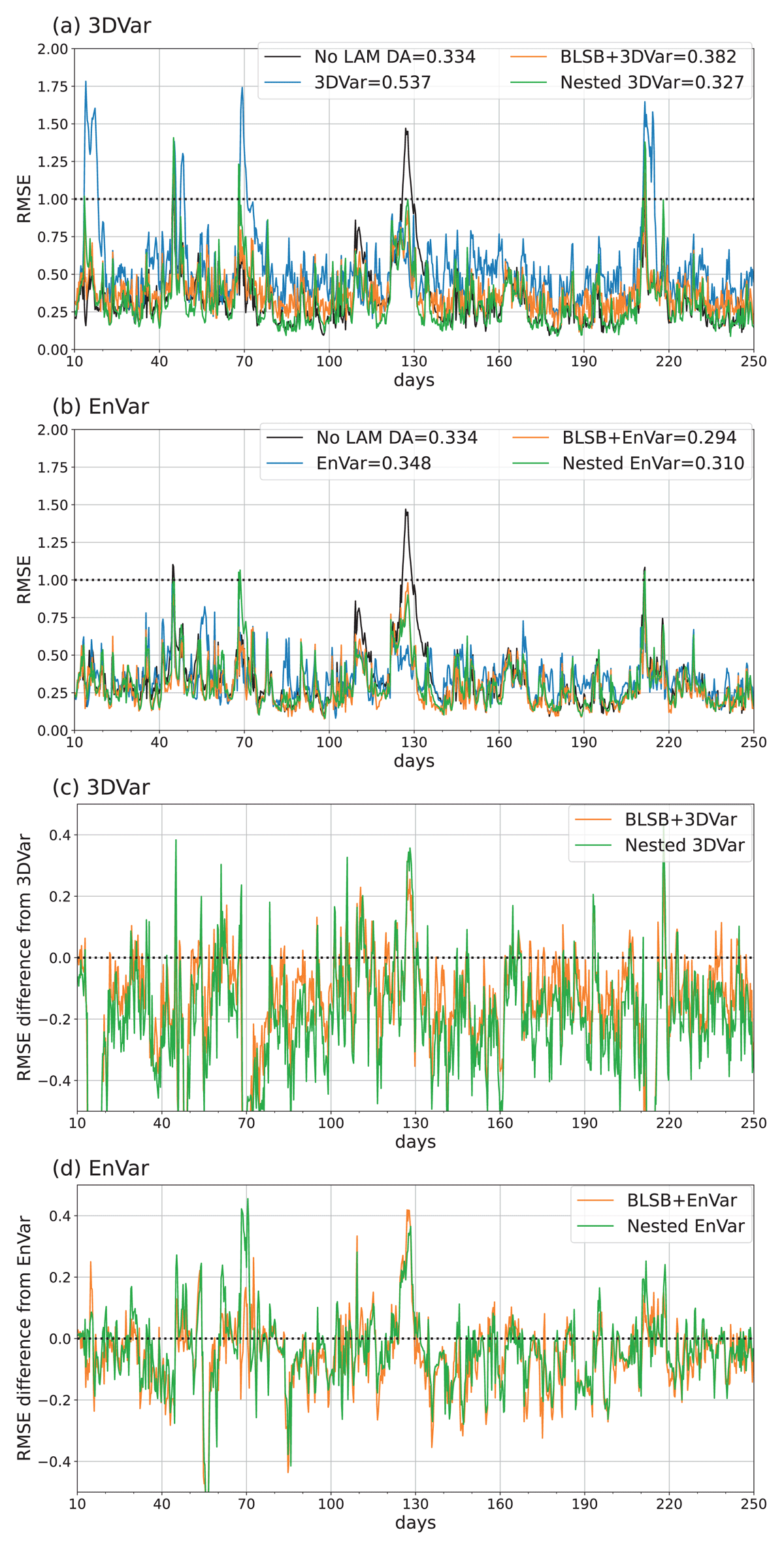
Figure 1
Time development of analysis RMSEs in the (a) 3DVar and (b) EnVar experiments with uniform observations. The values on the legend indicate time-averaged RMSEs. The dotted lines at RMSE = 1 indicate the standard deviation of the observation error, (c, d) as in (a, b), but for the differences from LAM DA for (c) 3DVar and (d) EnVar experiments.
The skill scores of the experiments without LSB (Table 2) show that LAM DA deteriorates over the large scale, which though consistent with previous studies (Berre, 2000; Guidard and Fischer, 2008; Baxter et al., 2011) improves the middle- to small-scale analysis. In No LAM DA, the error in large-scale structures (0.0987) accounts for approximately 65% of the overall error (0.151). The large-scale error is much more dominant (>90%) in the LAM DA experiments than in No LAM DA, suggesting that overall accuracy strongly depends on the accuracy of large-scale structures. In contrast to the significant degradation in the skill score of 3DVar, the skill score of EnVar is slightly positive, indicating that EnVar and No LAM DA show comparable performances. The flow dependency of the background errors considered in EnVar mitigates the large-scale deterioration caused by climatological background errors in 3DVar. This mitigation probably stems from the better representation of multi-scale error correlations in EnVar (Johnson et al., 2015). Nevertheless, the increases in large-scale errors are almost of the same magnitude as the decreases in middle- to small-scale errors caused by LAM EnVar, suggesting that the large-scale degradation in LAM DA can cancel the impact of the high-resolution LAM analysis upon the GM analysis.
Table 2
Skill scores of the analysis MSE and contributions of different scales in the experiments with uniform observations. Values in parentheses indicate the MSEs of No LAM DA.
| METHOD (MSEref) | ALL k (1.51e-01) | k ≤ 24 (9.87e-02) | k > 24 (5.22e-02) |
|---|---|---|---|
| 3DVar | –1.4 | –1.6 | 0.18 |
| BLSB+3DVar | –0.10 | –0.38 | 0.27 |
| Nested 3DVar | 0.052 | –0.22 | 0.27 |
| EnVar | 0.085 | –0.21 | 0.29 |
| BLSB+EnVar | 0.28 | –0.014 | 0.29 |
| Nested EnVar | 0.20 | –0.073 | 0.27 |
The introduction of LSB methods significantly improves the accuracies of the 3DVar and EnVar experiments. The impact of LSB methods on the analysis is highlighted by the differences in RMSE for BLSB+DA and Nested DA from LAM DA analyses (Figure 1c, d), where the negative difference presents improvement. In the 3DVar experiments with LSB (Figure 1c) the analyses are improved throughout the experimental period. Nested 3DVar achieves the most stable and accurate performance in the 3DVar experiments. The improvement effect of the LSB methods in the EnVar experiments is less impressive because EnVar is more accurate than 3DVar (Figure 1d). Nevertheless, the LSB methods improve the analyses over EnVar, mainly during the relatively accurate periods of No LAM DA (days 80–110 and 150–200, Figure 1d).
These improvements can be explained by the expected effect of LSB. Specifically, the LSB methods mitigate the large-scale worsening while retaining the accuracy on middle to small scales (Table 2). In the 3DVar experiments, BLSB+3DVar and Nested 3DVar reduce the analysis MSE by 53% and 60%, respectively, indicating that LSB significantly improves the analyses. This large error reduction is mainly attributable to improvement on the large scale but the error is also reduced on the middle to small scales. Therefore, the mitigation of large-scale errors by the LSB methods is beneficial to the performance of the LAM DA. In the EnVar experiments, BLSB+EnVar and Nested EnVar reduce the analysis MSE by 21% and 13%, respectively. BLSB+EnVar almost cancels the degradation of large-scale structures and highlights the impact of LAM DA, yielding a 28% MSE improvement over No LAM DA. Nested EnVar also mitigates the large-scale deterioration of EnVar, but worsens errors on middle to small scales relative to EnVar. Consequently, the MSE is 20% lower in Nested EnVar than in No LAM DA.
For a comprehensive comparison between the performances of the BLSB and our Nested EnVar we examine the analysis-error distributions in state space (Figure 2) and spectral space (Figure 3). The analysis error of No LAM DA is smaller and larger in the left () and right () parts of the LAM domain than the average, respectively (Figure 2). Given observations are assimilated regularly in the GM analysis, the spatial imbalance in accuracy is likely due to the chaotic nature of Lorenz models rather than the observations. The ensemble spread of No LAM DA is locally minimized at the observed locations and locally maximized between the observed locations. The analysis ensemble of No LAM DA is overconfident, meaning that the ensemble spread is smaller than the analysis error, and that the LAM DA tends to emphasize the background state over the observations. As indicated in the error spectrum of No LAM DA (Figure 3), the averaged errors are mainly contributed by large-scale errors (see also Table 2). The error in spectral space peaks near because the analysis error of No LAM DA tends to favor wavenumber-30 structures with the local minima at the observed evenly distributed locations (Figure 2).
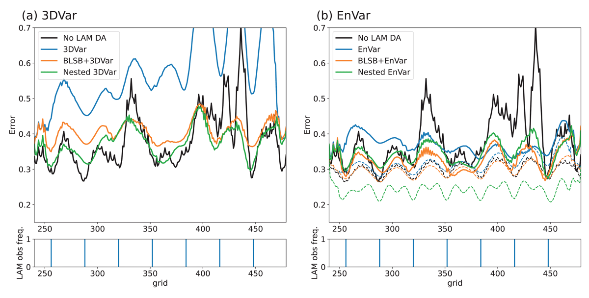
Figure 2
Time averaged analysis errors in state space: results of (a) 3DVar and (b) EnVar experiments with uniform observations. The dashed curves in (b) show the time averaged analysis spreads in each experiment. Observational frequency in LAM experiments is shown below each figure.
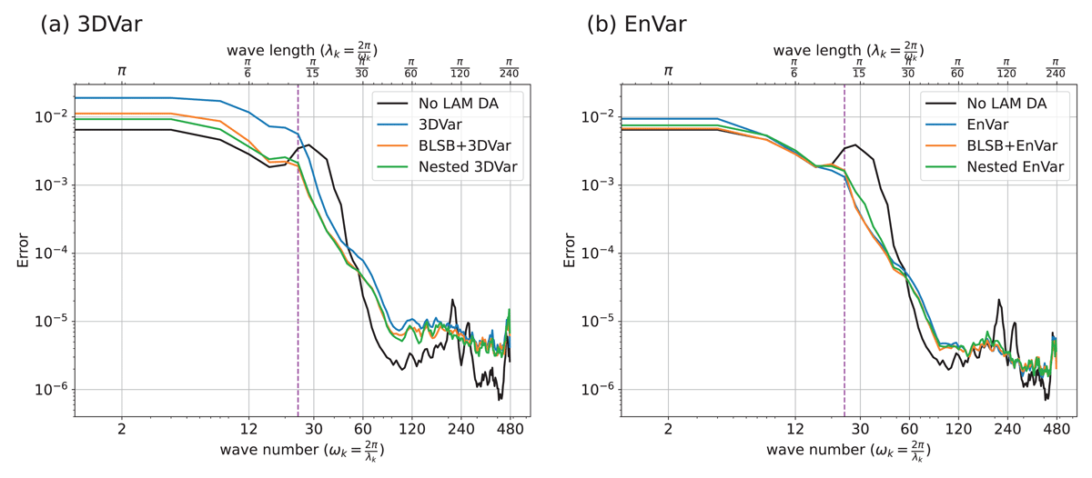
Figure 3
Time averaged analysis errors in spectral space: results of (a) 3DVar and (b) EnVar experiments with uniform observations. The bottom and top axes indicate the wavenumber and wavelength defined in the global domain, respectively. The vertical magenta lines indicate the truncation wavenumber in the LSB experiments.
Relative to No LAM DA, the analysis error in 3DVar (Figure 2a) increases more than that in EnVar, especially in the left part of the domain. The analysis error spectrum of 3DVar (Figure 3a) shows an obvious increase across the scales, obscuring the impact of DA over the middle wavelengths. After introducing the LSB, the analysis accuracy becomes comparable to that of No LAM DA, but the error in BLSB+3DVar exceeds that of No LAM DA because the large-scale structures are worsened by post-blending assimilation into the LAM (Figure 3a). By contrast, Nested 3DVar mitigates the deterioration of large-scale structures through the simultaneous assimilation of the observations and GM information (Figure 3a), thereby improving the analysis error in the left part of the domain from that of No LAM DA (Figure 2a). Whereas the GM reflects the flow dependency of the forecast errors represented by EnVar, the LAM DA depends on the static background errors in the 3DVar experiments. The inappropriate representation of background errors enlarges the analysis error from that of GM. Based on this example, it is suggested that the simultaneously incorporating the GM information into nested DA is beneficial when the GM and LAM DA systems clearly differ.
The accuracy of EnVar (Figure 2b) exceeds that of No LAM DA within a wide domain to the right of , but is reduced in the left part of the domain, which is accurately represented by No LAM DA. Given the slightly larger ensemble spread of EnVar in the right than in the left part of the domain, the accuracy imbalance can be attributed to overconfidence in the left part of the domain. The analysis error spectrum (Figure 3b) indicates apparent deterioration on the large scale (see also Table 2). The peak around seen in the error spectrum of No LAM DA is diminished in the spectrum of EnVar, indicating that the LAM DA mainly affects the scales around . BLSB+EnVar improves the analysis from that of EnVar in the left part of the domain because it incorporates the GM backgrounds (Figure 2b). By virtue of the high-resolution DA it also achieves higher accuracy than No LAM DA throughout the domain. The ensemble spread of BLSB+EnVar is smaller than that of EnVar and comparable to that of No LAM DA, but the underestimation of ensemble spread is relaxed because the reduction of analysis error is larger than that of the ensemble spread. The large-scale error magnitude almost matches that of No LAM DA in the analysis error spectrum (Figure 3b) and the middle-scale error magnitude around almost matches that in EnVar, which explains the smaller analysis error of BLSB+EnVar than in No LAM DA. Nested EnVar (Figure 2b) improves the analysis from that of EnVar in the left part of the domain, albeit to a smaller extent than BLSB+EnVar, and slightly degrades the analysis error in the right part of the domain. The analysis error of Nested EnVar resembles that of No LAM DA throughout the domain, clarifying the influence of simultaneously assimilating the GM information and observations. Incorporating the GM information into the analysis increases the amount of information, as the reduction of the ensemble spread is larger than in the other experiments (Figure 2b). The distribution of ensemble spreads is locally minimized not only at the observed locations as in the other experiments, but also at the grids of low-resolution LAM space (corresponding to the middle of the observed locations). The larger underestimation of ensemble spread in Nested EnVar than in EnVar reduces the influence of observations on the analysis. Therefore, the analysis state should be similar to that in No LAM DA. The analysis error spectrum of Nested EnVar (Figure 3b) is slightly increased on the large scale caused by underestimation of the observational influence. Reflecting the large resemblance of Nested EnVar to No LAM DA, the analysis error in the middle scale (around ) is also larger than in EnVar and BLSB+EnVar. These results indicate that both BLSB+EnVar and Nested EnVar mitigate the large-scale deterioration in LAM DA, but in Nested EnVar the underestimated ensemble spread must be alleviated to adequately represent the balance between the LAM background, observations and large-scale GM errors. Note that unlike the analysis error spectrum of Nested EnVar, the spectrum of Nested 3DVar (Figure 3a) shows no obvious error increases near , probably because the information in the static large-scale GM error covariance excludes the error peak at in the GM analysis.
Comparing errors in the analysis, LSB methods are found to be important in improving the performance of LAM DA over that of GM analysis, which is consistent with previous studies. To examine the contribution of analysis-accuracy improvement by the LSB methods in forecasting, Figure 4 compares the RMSEs in the extended forecasts from each analysis. To show the forecast errors introduced through the LBCs of the LAM, the errors of the GM forecasts within the LAM domain are also plotted. The slightly faster forecast error growth in Dscl than in GM is attributable to the artificial LBCs. All LAM DA experiments except 3DVar show a faster forecast error growth than Dscl. The forecast error amplitudes of LAM experiments approximately double in 24 hours, which is consistent with the estimated doubling time of Lorenz III. Initially, the RMSE is lower in Nested 3DVar, BLSB+EnVar, and Nested EnVar than in Dscl, although the improvement is significant (p < 0.05) only in BLSB+EnVar and Nested EnVar. The forecast errors of Nested EnVar approaches those of Dscl after six forecasting hours (FT6) and exceeds those of Dscl after FT18 (Figure 4b). By contrast, BLSB+EnVar achieves a smaller forecast error than Dscl (p < 0.05) until FT24 (Figure 4b). Although the forecast error grows slightly faster in BLSB+EnVar than that in Nested EnVar, the larger improvement at the initial time extends the lead time from that of Nested EnVar. The ensemble forecasts present similar error growths to the deterministic forecasts, and the initial underestimation of ensemble spread in EnVar and Nested EnVar remains until FT48 (not shown).
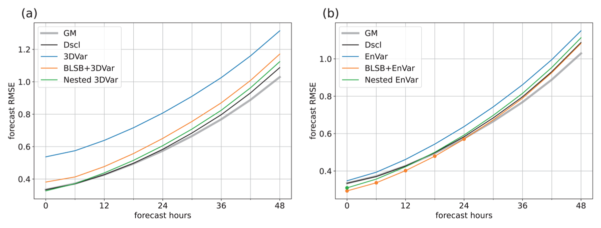
Figure 4
RMSE of deterministic forecasts from the (a) 3DVar and (b) EnVar experiments with uniform observations. Each curve is averaged over the assimilation cycles. Circles indicate a significant improvement over downscaling (p < 0.05). Thicker gray curves show the forecast RMSEs of the GM within the LAM domain. Horizontal axes indicate hours from the analysis time.
The results of Exp. 1 confirm that nested EnVar can alleviate large-scale errors for conventional LAM DA as for existing LSB methods. Our proposed Nested EnVar shows higher accuracy than Nested 3DVar, and comparable performance to BLSB+EnVar, however, Nested EnVar tends to be more overconfident than EnVar and BLSB+EnVar because it enlarges the reduction of the analysis ensemble spread, thus shortening the lead time against the dynamical downscaling of GM from that of BLSB+EnVar. The current covariance inflation rate in Nested EnVar is adjusted to minimize the analysis RMSE. Although increasing the inflation rate reduces the underestimation of the spread, it increases the analysis RMSE (not shown). Because the analysis ensemble perturbations in Nested EnVar are updated by Eq. (30), incorporating the large-scale GM information will likely reduce the large-scale ensemble spread. To minimize analysis error while ensuring an adequate ensemble spread we are required to introduce scale-dependent covariance inflation, which is beyond the scope of this study.
5 Sensitivity to the Observation Network
This section investigates the impact of nested EnVar on the analysis and forecast performance when observations assimilated by LAM DA differ from those in the global analysis.
Table 3 shows the analysis RMSEs in the experiments on dense, uneven observation networks (Exp. 2–5). Only the skill scores for Exp. 5 are shown in Table 4 since the trends of the scores are similar in Exp. 2–5. Although these experiments assimilate more observations than Exp. 1, all the conventional LAM DA without LSB methods (except EnVar in Exp. 5) generate larger analysis RMSEs than Exp. 1. Especially, the analysis errors of 3DVar are significantly worsened from the observation error when only part of the domain is observed. The comparison of the skill scores between uniform (Table 2) and uneven (Table 4) observations clarifies that this significant degradation is mainly caused by the increase of the large-scale errors, indicating that the large-scale structures are prone to disturbance through the uneven observations caused by the unbalanced analysis accuracy across the domain. Note that there are differences in accuracies of both 3DVar and EnVar between the observation networks in the left (Exp. 2) and right (Exp. 4) parts of the LAM domain (Table 3). The analysis RMSE of 3DVar is smaller with observations in the left than in the right, since the group velocity of Lorenz III tends to propagate the observational information to the right (Yoon, Ott, and Szunyogh, 2010). Although the rightward propagation of the observational information is also seen in EnVar, EnVar tends to show large errors in the right part of the LAM domain as seen in Figure 2, and EnVar with the observations in the right reduces these errors more effectively than with the observations in the left.
Table 3
Time averaged analysis RMSEs in the experiments with dense and uneven observations.
| METHOD | EXP. 2 | EXP. 3 | EXP. 4 | EXP. 5 |
|---|---|---|---|---|
| 3DVar | 3.29 | 1.33 | 3.34 | 0.652 |
| BLSB+3DVar | 0.331 | 0.327 | 0.328 | 0.329 |
| Nested 3DVar | 0.323 | 0.313 | 0.323 | 0.311 |
| EnVar | 0.662 | 0.371 | 0.543 | 0.315 |
| BLSB+EnVar | 0.295 | 0.285 | 0.291 | 0.283 |
| Nested EnVar | 0.287 | 0.273 | 0.307 | 0.258 |
Table 4
As for Table 2, but in the experiments with dense and uneven observations moving in the LAM domain (Exp. 5).
| METHOD | ALL k | k ≤ 24 | k > 24 |
|---|---|---|---|
| 3DVar | –4.7 | –4.5 | –0.17 |
| BLSB+3DVar | 0.086 | –0.19 | 0.27 |
| Nested 3DVar | 0.13 | –0.15 | 0.27 |
| EnVar | 0.15 | –0.15 | 0.29 |
| BLSB+EnVar | 0.30 | 0.014 | 0.29 |
| Nested EnVar | 0.40 | 0.11 | 0.29 |
LSB methods largely mitigate large-scale deterioration and reduce the sensitivity of analysis to observation networks (Table 3). In particular, the increased number of observations yields better analysis accuracy in BLSB+3DVar and Nested 3DVar than of Exp. 1. In both the 3DVar and EnVar experiments, the performances of BLSB+DA and Nested DA do not significantly differ in the dense observation networks in the left, center, and right parts of the LAM domain (Table 3). It should be noted that on the right-sided observation network, Nested EnVar obtains a slightly larger RMSE and lower skill score than BLSB+EnVar, reflecting the higher susceptibility of Nested EnVar than of BLSB+EnVar to the GM characteristics of the large errors at the right domain side (Figure 2). Alleviating the spread underestimation might reduce this accuracy difference as discussed in Section 4.
In the experiment with mobile observations (Exp. 5, Table 4), Nested DA outperforms BLSB+DA in terms of both performance measures (analysis RMSE and skill scores). Although the analysis RMSEs of Nested 3DVar and BLSB+3DVar are closer in Exp. 5 than in Exp. 1, those of Nested EnVar and BLSB+EnVar are more separated than in Exps. 1–4 and the difference is statistically significant (p < 0.01). This result suggests that the flow-dependent Nested DA is more suitable for dense and mobile observations than BLSB+DA. Hereafter, we focus on the results of Exp. 5 in EnVar.
The RMSE of EnVar spikes more frequently in Exp. 5 than in Exp. 1 (Figure 5a) although the time-averaged RMSE is reduced (0.315 vs 0.348), suggesting that the analysis is destabilized by uneven observations. Introducing LSB methods extends the accurate and stable period from that of Exp. 1 but does not remove all RMSE peaks. In general, Nested EnVar achieves a lower RMSE than EnVar and BLSB+EnVar during the stable period (days 80–90 and 150–200, Figure 5b).
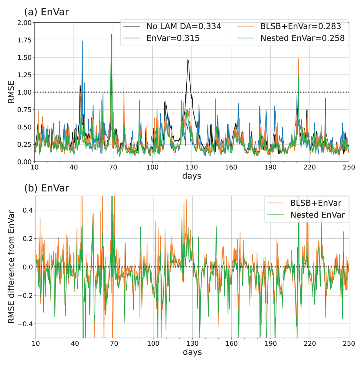
Figure 5
As for Figure 1b, d, but obtained in experiments with dense, mobile observations.
The analysis error of EnVar is lower in Exp. 5 than in Exp. 1 in the right part of the domain, with the spread also decreasing owing to the increased number of observations (Figure 6a); thereby EnVar becomes overconfident as observed in Exp. 1. BLSB+EnVar relaxes the underestimation of the ensemble spread, as also observed in Exp. 1, but the analysis accuracy is not clearly improved from that of Exp. 1. In contrast, Nested EnVar improves the analysis in all parts of the domain except the near-boundary parts. Like EnVar, Nested EnVar decreases the ensemble spread, but the obvious wave-like structures observed in Figure 2b are diminished by the uneven observations.
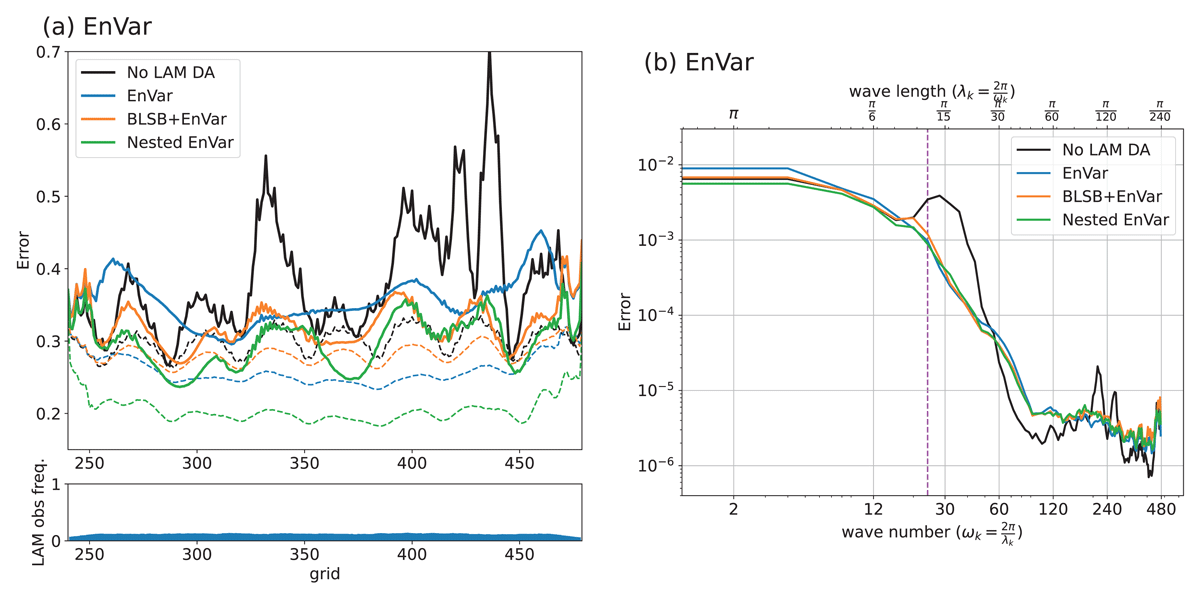
Figure 6
As for (a) Figure 2b and (b) Figure 3b, but obtained in experiments with dense, mobile observations.
As indicated in the analysis error spectrum (Figure 6b), EnVar performs slightly better in Exp. 5 than in Exp. 1 (Figure 3b), even though the large-scale error still increases relative to that of No LAM DA. The error spectrum of BLSB+EnVar almost coincides with that of No LAM DA on scales larger than the truncation wavelength of LSB, consistent with the minimal improvement (~1%) in the large-scale component of the skill score (Table 4). Nested EnVar reduces the analysis error across a wide range of wavelengths (from to ). The error peak around in Figure 3b, remains in Figure 6b but is less obvious because more observations are assimilated in the LAM domain. In particular, Nested EnVar obtains a comparable analysis error to EnVar and a smaller analysis error than BLSB+EnVar around , indicating that Nested EnVar appropriately incorporates the information of both GM and LAM background errors.
The deterministic forecasts of BLSB+EnVar and Nested EnVar are significantly improved (p < 0.05) from those of Dscl until FT30 and FT36, respectively (Figure 7b). The extended lead times in both experiments are attributable to improvement of the initial analysis because the forecast error grows by almost the same rate in Exps. 5 and 1 (Figure 4). The ensemble forecasts of Nested EnVar are also significantly improved up to FT36 (not shown). Although Nested 3DVar outperforms BLSB+3DVar, the improvement is statistically significant only up to FT6 (Figure 7a), suggesting that the flow dependency of background errors is important for effectively assimilating dense observations into LAM.
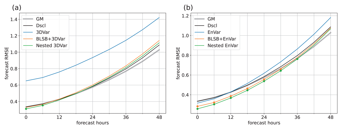
Figure 7
As for Figure 4, but obtained in experiments with dense, mobile observations.
6 Discussion and Conclusion
In this study, to alleviate the large-scale deterioration problem in LAM DA, we proposed a novel flow-dependent nested DA scheme that introduces large-scale GM information into an EnVar-based LAM analysis. The proposed nested EnVar can dynamically incorporate large-scale GM information by weighting the large-scale information relative to LAM backgrounds and observations. The weights are determined with consideration of both the GM and LAM flow-dependent background errors. The impact of blending timing and flow dependency on the LSB methods was clarified through direct performance comparisons of the nested EnVar, the BLSB method, and the static nested DA proposed in aforementioned previous studies.
The performances of LSB methods were evaluated through idealized cycled experiments, using the spatially one-dimensional chaotic models of Lorenz (2005). Both BLSB and nested DA mitigated the large-scale analysis errors introduced by LAM DA, but the blending timing affected the performance of the 3DVar experiments. Because the GM EnVar was generally more accurate than the LAM 3DVar, simultaneous assimilation of the GM information with observations by the nested 3DVar more effectively mitigated large-scale errors than GM blending prior to DA by the BLSB method. EnVar with the flow-dependent background error covariance can partly reduce the large-scale degradation from that of 3DVar with static background error covariance. Nevertheless, as large-scale structures generally have higher energy than small-scale structures, the deterioration on large scales is still serious and negates the positive impact of LAM DA on the middle to small scales. Therefore, both the BLSB method with EnVar and our proposed nested EnVar benefit the analysis and forecast by alleviating the large-scale errors, achieving higher analysis accuracy than interpolating the GM analysis. Although the spread reduction tends to be larger in nested EnVar than in the BLSB method with EnVar, the difference in blending timing has less influence on the performances of LSB methods with EnVar than with 3DVar. These results suggest that simultaneous assimilation by nested DA methods has an advantage over background blending when LAM DA is known to introduce severe large-scale errors into the analysis.
Furthermore, the flow-dependent LSB method exerts a large influence when assimilating uneven observations into LAM because such observations more likely introduce inhomogeneity in LAM analysis accuracies than the uniform observations. Our nested EnVar significantly outperforms the other LSB methods when assimilating dense, uneven observations moving across the LAM domain. By considering the flow-dependent GM background errors, the nested EnVar can appropriately balance the large-scale constraint with the DA impact on middle to small scales, enabling accurate analyses across the scales. Therefore, dynamical large-scale blending, taking into account the flow dependency of background errors, is likely to be beneficial, especially when assimilating dense, spatially localized observations such as microwave sounders. Judging from these encouraging results, the nested EnVar is a promising alternative to current LSB methods.
However, several challenges in the nested EnVar must be resolved. First, the underestimation of the ensemble spread relative to the analysis or forecast error is more severe in the nested EnVar than in the EnVar and EnVar with BLSB, weakening the impact of assimilation in the experiment with the uniform observations. To reflect the GM error information on the analysis ensemble perturbations, the nested EnVar updates the ensemble with the Hessian of the cost function (Zupanski, 2005), which more enlarges the reduction of the analysis spread, especially on large scales, than the traditional ensemble update considering only the observational information. The current covariance inflation, which assumes a constant inflation rate on all scales, cannot adjust the ensemble spread on each scale. The impact of scale-selective inflation on the nested EnVar will be investigated in future work.
In addition, like the formulations of GF08 and DG12, the formulation of nested EnVar ignores the correlation between the GM and LAM background errors. Some correlation between these errors is expected because GM and LAM connects at lateral boundaries. The cross covariance between the background errors of GM and LAM can be estimated using Monte–Carlo methods similar to autocovariances, however incorporating the cross covariance in EnVar requires the approximate inverse calculation of a huge matrix. If the ensemble size is far smaller than the degree of freedom in state space, the two background errors can be regarded as maximally correlated (Berry and Sauer, 2018) even when not strictly true. This situation causes an excessively high condition number for the huge matrix, destabilizing the numerical optimization and hindering proper evaluations of the GM background error. To incorporate the cross covariance between background errors, we require methods or assumptions that overcome the rank-deficient problem.
Such a rank-deficient problem might also arise when applying the nested EnVar to high-dimensional realistic models. In ensemble data assimilation, the rank-deficient problem is commonly compensated with well-established localization, but the performance of this approach strongly relies on localization cut-off scales. If the observation space localization (Hunt, Kostelich, and Szunyogh, 2007) is applied to the nested EnVar, the GM information must be localized based on the distance from a model grid similar to observations. The localization cut-off scale of the GM information is expected to be longer than that of the observations. If the GM background errors are localized in state space (Zupanski, 2021), different cut-off scales may be required for the GM and LAM background ensembles. To effectively introduce localization to the nested EnVar we should define or estimate localization functions with proper cut-off scales for both GM and LAM. Along with the inflation problem, appropriate localization schemes for the nested EnVar will be considered in future work.
Data Accessibility Statement
The source code is available from https://github.com/s-nakashita/pydpac.
Acknowledgements
The authors greatfully appreciate the anonymous reviewer for the constructive comments and encouraging suggestions. The authors thank Dr. Yosuke Fujii and Dr. Daisuke Hotta for helpful discussions.
Competing Interests
The authors have no competing interests to declare.
Author Contributions
Saori Nakashita made conceptualizations, developed the code, conducted all the experiments, and wrote the main text. Takeshi Enomoto suggested experimental designs and contributed to the interpretation of the results.