
1 Introduction
The Arctic Ocean, which in the established hydrographic definition includes the Nordic Seas (Jakobsson, 2002), is in terms of area the smallest of Earth’s ocean basins. Even so, the landlocked Arctic Ocean harbours a range of oceanographic conditions which are influenced by exchanges with the Pacific and Atlantic Oceans, continental runoff and a perennial sea-ice cover (Rudels et al., 2012; Haine et al., 2015; Timmermans and Marshall, 2020). The Arctic Ocean is one part of the climate system that has responded strongly to global warming (Previdi et al., 2021), and where pronounced sea-ice cover retreat and changes in upper ocean hydrography have been observed (Carmack et al., 2015; Ingvaldsen et al., 2021).
Climate change in the Arctic Ocean has contributed to an increased interest in exploring the fundamental dynamics of its circulation and how it interacts with the sea-ice cover, adjacent ocean basins and the overlaying atmosphere (Timmermans and Marshall, 2020). These efforts have so far faced the challenge of a data scarcity and a partial lack of a theoretical framework for understanding the dynamics. In the subtropical and subpolar oceans the Sverdrup relation (Sverdrup, 1947) provides a corner stone for the wind-driven gyre circulation (Gill, 1982; Rhines and Young, 1982). However, in the Arctic Ocean as well as in the Southern Ocean, where closed contours of f/H are encountered, the Sverdrup relation no longer governs the leading order wind-driven circulation.
In regions with closed f/H contours, wind forcing tends to primarily drive flows along those contours, rather than across them, and Ekman and eddy-induced flows control the transport across the f/H contours (Greenspan, 1968; Johnson and Bryden, 1989; Marshall and Speer, 2012; Timmermans and Marshall, 2020). In the Arctic Ocean, where the f/H contours are dominated by the variations in depth, the time-mean bottom currents are expected to be aligned with the depth contours (Nøst and Isachsen, 2003; Yang et al., 2016; Broomé and Nilsson, 2016). This is because even small cross bottom-slope velocities would induce strong vertical velocities which cannot be balanced by horizontal divergence or convergence in a nearly geostrophic flow (Greenspan, 1968).
Although the near surface flow is not directly constrained, dynamically, by the bottom topography, observations show that the time-mean surface currents in the Arctic Ocean tend to be aligned with the depth contours (see e.g., Woodgate et al., 2001; Jakobsen et al., 2003; Nilsson et al., 2008; Koszalka et al., 2011; de Steur et al., 2014; Broomé and Nilsson, 2016; Armitage et al., 2017). This tendency can be seen, for example, in satellite-altimetry based surface currents: Figure 1 shows a measure of the alignment between the time-mean altimetry-estimated surface flow and the topography defined by
where uS is the surface velocity and a unit vector along the topography directed with shallow water to its right; here, k is the vertical unit vector. Note that α is the angle between the surface velocity and the depth contour, and as defined here cos(α) is 1 (–1) when the flow is perfectly aligned with the bathymetry and moves with shallow water to the right (left). An inspection of Figure 1 reveals that the surface currents tends to be aligned with the bathymetry which corresponds to values of cos(α) that are near 1 or –1. It is less common to encounter surface flows oriented perpendicular to the depth contours, corresponding to cos(α) ≈ 0. It is also clear that the time-mean surface flow is mainly cyclonic in the Nordic Seas and the Eurasian Arctic Basin whereas the flow is mostly anticyclonic in the Amerasian Arctic Basin.
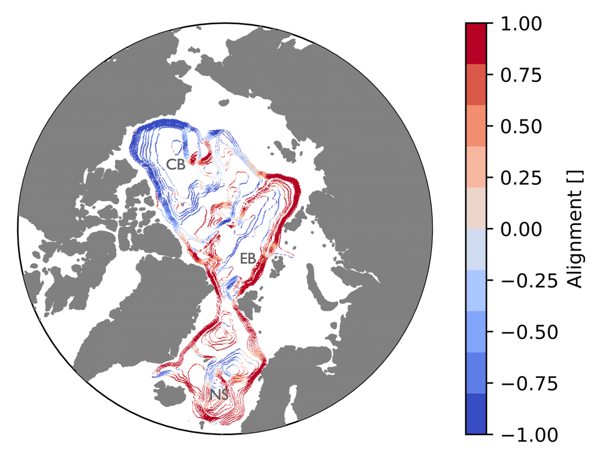
Figure 1
Alignment of the time-mean surface flow with the bathymetry; the surface flow is based on satellite altimetry (Mulet et al., 2021). Here, the alignment is defined as the cosine of the angle between the surface flow and the depth contours; see Eq. (1). Positive (negative) values show flow with shallow water to the right (left). The figure shows the alignment along selected depth contours in the range ∼800–4000 m; the Canada Basin (CB), the Eurasian Basin (EB) and the Norwegian Sea (NS) are indicated. The ∼ 800 m depth contour separates between shallow contours, extending into the Atlantic, and deeper locally closed contours. The bathymetry has been smoothed with a filter that suppresses variation on scales below around 100 km. For a flow field that is randomly oriented relative to the bathymetry the angle α will be uniformly distributed between 0 and 2π; in this case the mean of |cos(α)| is π/2 ≈ 0.6. Similar results are obtained on f/H contours (not shown). Note that the Transpolar Drift, directed from CB towards EB, crosses topography in the Central Arctic Basin (Rudels et al., 2012; Haine et al., 2015; Timmermans and Marshall, 2020).
To examine dynamics that can cause the time-mean surface flow to be aligned with the topography we will use a two-layer model that incorporates elements from existing models of wind-driven Arctic Ocean circulation. For simplicity the f-plane approximation is made. Following Nøst and Isachsen (2003), the lower layer flow on closed depth contours is determined by an integral balance between surface wind stress and bottom friction stress. The upper layer thickness is forced by surface Ekman pumping and modulated by diffusion of upper layer thickness, representing the collective effect of mesoscale eddies (Marshall et al., 2002; Manucharyan and Spall, 2016; Manucharyan et al., 2016) as well as advection directed preferentially along the isobaths.
In addition to local wind-forcing, the exchange of water masses across the Greenland–Scotland Ridge contribute in forcing the circulation in the Arctic Ocean (Hansen and Østerhus, 2000; Rudels et al., 2005). This component of the circulation is maintained by large-scale gradients in surface buoyancy forcing and associated with water mass transformations of poleward flowing Atlantic Water (Walin et al., 2004; Isachsen and Nøst, 2012; Spall, 2013). We will use the two-layer model to examine how local wind forcing and forced Atlantic Water inflow across the Greenland–Scotland Ridge influence the interplay between the flow and topography: In the eastern Nordic Sea there is a general poleward flow of Atlantic Water in the upper ocean that to some extent crosses closed isobaths in the local deep basins. What mechanisms can cause topographic alignment of the Atlantic surface flow in this setting?
The presentation is organised as follows. In section 2 and 3 the model, scaling analyses and non-dimensional parameters are presented. Model solutions representing different Arctic Ocean regimes are derived in section 4 and discussions and conclusions are presented in section 5. Some mathematical derivations are given in the appendix.
2 A Two-Layer Model
2.1 Governing equations
We develop a two-layer model to examine the large-scale circulation in the Nordic Seas and the Central Arctic Ocean. For simplicity we use the f-plane approximation. We focus on the time-mean circulation and variations of the circulation on seasonal and inter-annual timescales. The model describes the flow averaged over a spatial scale that well exceeds the baroclinic Rossby radius and assumes that the leading order flow is in geostrophic balance. Different from the standard quasi-geotropic approximation, however, the model does not require variations in the interface-layer and total depths to be on the order of the Rossby number (see e.g. Allen, 1991). Although formulated on an f-plane the model accordingly shares some features with the planetary geostrophic approximation which includes the advection of the entire buoyancy field (Welander, 1959). The model does not resolve baroclinic eddies but their effect is represented as a diffusion of the upper-layer thickness which reduces its slope and thereby the baroclinicity of the flow. The thickness diffusion, which is equivalent to diffusion of the upper-layer planetary potential vorticity, can alternatively be interpreted as a form drag between the two layers caused by the baroclinic eddies. Potential effects of eddy-induced relative vorticity fluxes are not represented. Further, effects of surface wind forcing and bottom friction are modeled as surface and bottom Ekman transports in the continuity equation. The model includes elements of previous models of Arctic Ocean dynamics (Nøst and Isachsen, 2003; Manucharyan and Spall, 2016; Manucharyan et al., 2016; Meneghello et al., 2020), as will be discussed below.
Figure 2 shows the structure of the two-layer model, with the upper and lower depths denoted by H1 and H2, respectively. Note that the layer thicknesses H1 and H2 are not allowed to vanish. We assume that the large-scale flow is in geostrophic balance
where f is the Coriolis parameter, k the vertical unit vector and φ1 and φ2 are the dynamic pressures. The pressure is hydrostatic and the dynamical pressures in the two layers and the upper-layer thickness are related as
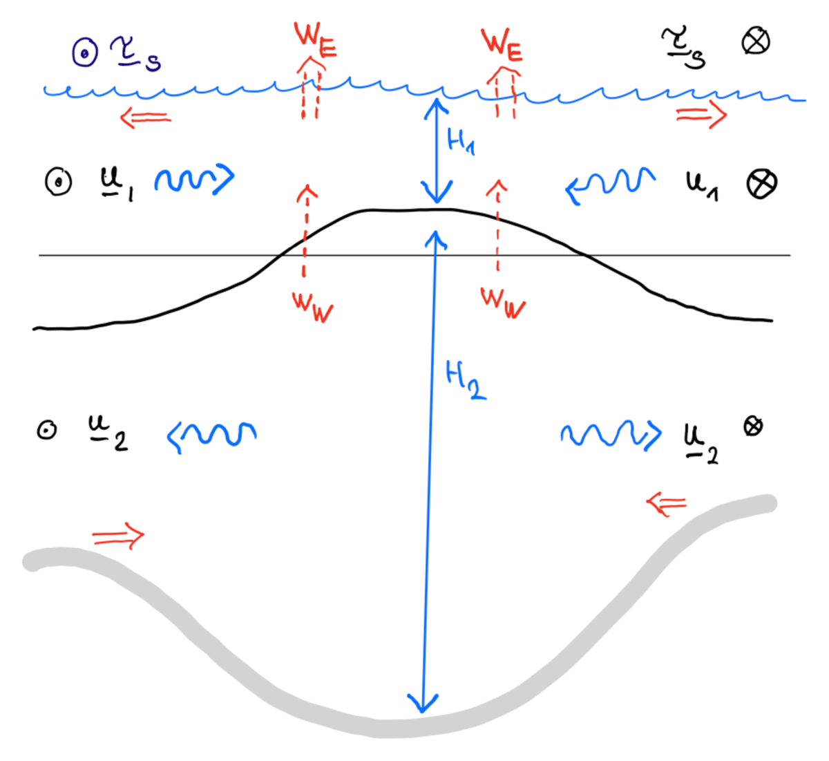
Figure 2
The two layer model, with subscript 1 (2) denoting the upper (lower) layer. The rigid lid approximation (Gill, 1982) is made and the total depth is time independent. The dynamic pressure in the layers are related as (Eq. 4) where φ1 is proportional to the sea surface height anomaly which is much smaller than the variations in H1. The red horizontal arrows show Ekman transports in the surface and bottom layer, respectively, and the blue wavy arrows show eddy-induced volume transports that are proportional to |∇H1|; see Eqs. (6,7). The red dashed vertical arrows represent wind-forced vertical Ekman velocity (wE) and transfer between the layers (wW) due to diabatic processes. The surface Ekman suction/pumping velocity wE and wW force the upper layer in similar ways (Eq. 15).
Here g′ is the reduced gravity and g′H1 is the baroclinic pressure anomaly. By using Eqs. (2–4) the layer velocity difference can be written as
This is the thermal wind velocity relative to the lower layer velocity and it is parallel to contours of H1.
We consider a flow with a scale that is much smaller than the barotropic Rossby radius which allows the free surface to be regarded as a rigid lid (Gill, 1982). The continuity equations include the vertically-integrated geostrophic transport, Ekman transports associated with surface and bottom stress, and eddy-induced transport represented as a thickness diffusion, or a bolus transport (Rhines and Young, 1982; Manucharyan et al., 2016; Meneghello et al., 2020). The vertically-integrated transports in the layers are
Here, K is the eddy diffusivity, –/+ K∇H1 the bolus transport in the upper/lower layer, τS the surface ocean stress and τB the bottom stress, which is represented as a linear drag
where R is a constant friction parameter. The continuity equations are then
Here, wW represents water-mass transfer between the two layers of different densities due to diabatic processes such as interior mixing and surface buoyancy fluxes (Walin, 1982). For surface forcing wW equals the surface buoyancy flux divided by g′ and is positive (negative) when the ocean gains (loses) buoyancy; e.g. surface cooling and associated densification of the surface layer may be represented as a volume transfer from the upper to the lower layer. Similarly, vertical mixing in the stratified interior of the ocean may be modelled as a cross interface volume transfer in a layered model (see e.g. Kawase, 1987; McDougall and Dewar, 1998). We will not here explicitly consider effects of diabatically forced wW but we include this term in the model formulation since surface buoyancy fluxes in parts of the Arctic Ocean may represent a forcing comparable to the wind-driven Ekman surface vertical velocity. For instance, along the Barents Sea Opening and in the West Spitzbergen Current where the surface buoyancy loss is intense (see Figure 3 in Isachsen et al., 2007) wW may be on the order of 10–6 m s–1, which is comparable to typical vertical surface Ekman velocities in the Arctic Ocean (Timmermans and Marshall, 2020).
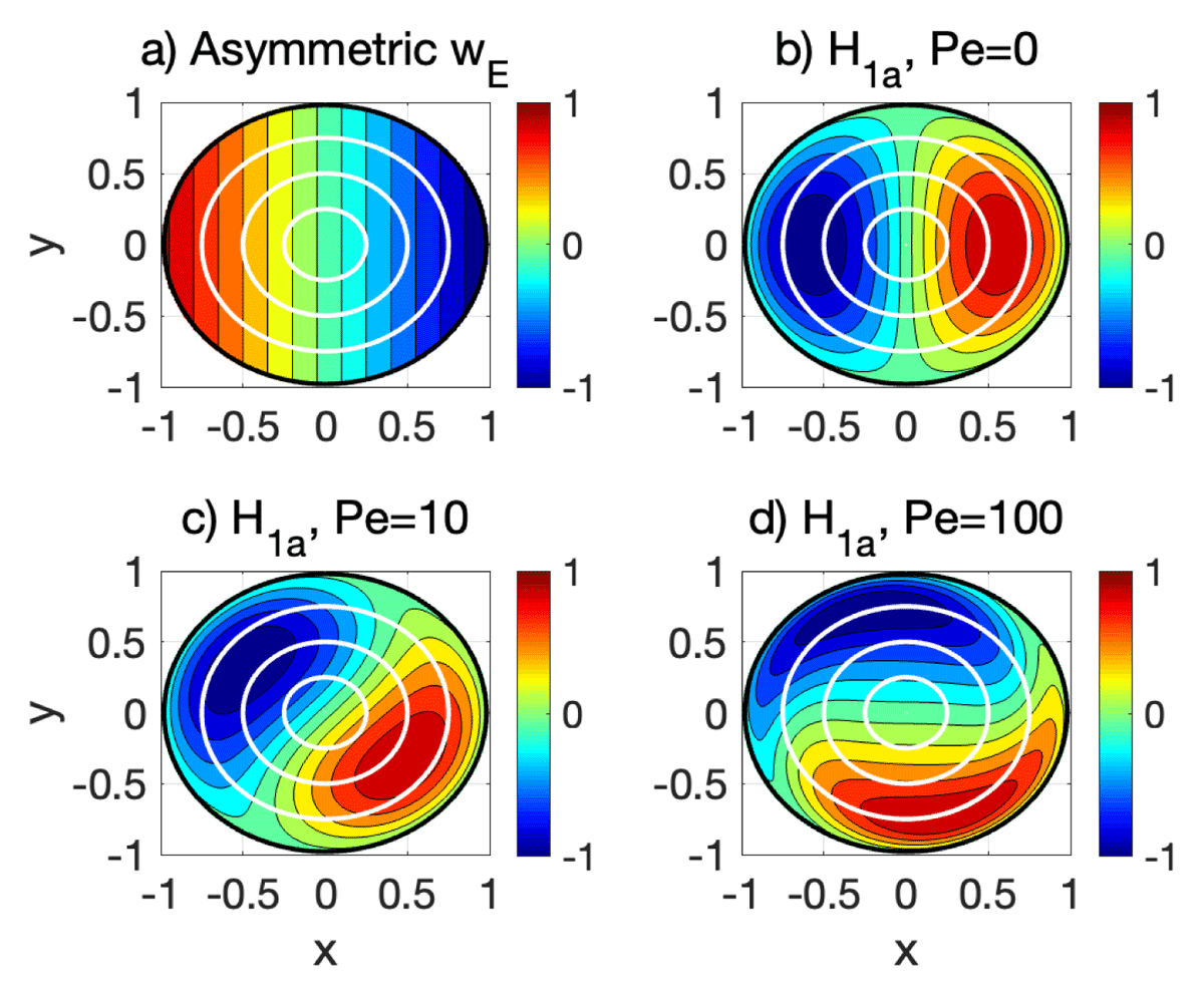
Figure 3
Pattern of asymmetric Ekman pumping [Eq. (42)] (a) and associated asymmetric upper-layer thickness H1a(r,θ) for varying Peclet numbers (b–d): Pe = 0 (b), Pe = 10 (c), and Pe = 100 (d). Here H1a is approximated by the first 50 terms in the infinite series defined by Eq. (A20). The amplitude of H1a(r,θ) decreases with Pe but is here normalised to range between –1 and +1. The white lines indicate circles () that coincide with the depth contours.
Since the geostrophic velocities are non divergent on an f plane, the continuity equations can be written as
Here, we have introduced the surface vertical Ekman velocity
and the depth of the bottom Ekman layer
Note that is the bottom vertical Ekman velocity which is upward (downward) for cyclonic (anticyclonic) lower-layer flow.
On the lateral boundaries of the model the normal components of the volume transports M1 and M2 (Eqs. 6, 7) need to be specified; we will return to this when specific solutions are considered.
2.2 Summary of governing equations
A convenient way to the describe the present two-layer system is in terms of the upper-layer continuity equation and the vertically-integrated continuity equation, obtained by adding Eqs. (11) and (12). By noting that is independent of time and that Eq. (5) implies that (i.e., the thermal wind velocity is parallel to H1), these equations can be written as
Equation (16) is essentially the two-layer and f-plane equivalent of the bottom-velocity equation used by Nøst and Isachsen (2003). Given the wind forcing, this linear equation yields , which allows us to solve the advective-diffusive equation for H1 (Eq. 15). Despite that the term formally is nonlinear, the upper-layer thickness is governed by a linear equation. A similar feature emerges in the beta-plane two-layer model considered by Rhines and Young (1982), for which the depth-integrated flow equation is also linear. We note that the diabatic volume transfer wW and the Ekman pumping wE both force the upper-layer thickness. However, wW does not affect the vertically-integrated continuity equation.
A noteworthy feature is that Eqs. (15,16) only involve the variations in upper-layer thickness and total depth; the average values of these quantities do not enter explicitly. Thus, there is no restriction that the variations of these variables should be small compared to their mean values, which is the case for the standard two-layer quasi-geostrophic model (Pedlosky, 1987; Allen, 1991). However, the Rossby number [U/(fL)] based on the thermal wind velocity (Eq. 5) is required to be small to ensure a leading-order geostrophic flow, which puts an upper limit on the upper layer slope |∇H1|. For the present Arctic Ocean application (Table 1) this requires that . Furthermore, the mean depth of the layers enter in the layer transports (Eqs. 6,7) and they also set the (two-layer) internal Rossby radius (Gill, 1982), which in turn can affect the eddy diffusivity K (Visbeck et al., 1997; Karsten et al., 2002). We emphasise that the present model does not predict the mean upper-layer thickness which has to be inferred from additional assumptions or observations. For the main aspects of our study, however, the mean upper-layer thickness does not matter.
2.3 Integral relations for the bottom flow over areas bounded by H contours
In the Arctic Ocean the depth contours deeper than about 800 m close themselves within the basin. On such closed depth contours the bottom flow is essentially governed by an integral momentum balance: From Eq. (16) we can derive the Nøst and Isachsen (2003) integral balance for our two-layer and f-plane model. To this end, we integrate Eq. (16) over an area A(H) enclosed by a curve C(H) defined by the depth contour H. By using Gauss’ theorem on the first term in Eq. (16) we obtain
Here n is a vector normal to C and ds the length element along C. The geostrophic balance (Eq. 3) yields , implying that the first term on the lefthand side integrates to zero since H/f is constant on C. By using Stokes’ theorem, Eq. (17) can then be written as
where is the vector length element along C, or alternatively since as
This shows that integrated around a closed depth contour, the Ekman transports in the surface and bottom layers are equal but of opposite signs. As f is constant this means that a bottom flow is established, associated with a bottom stress that balances the wind stress when integrated around a closed contour. Note that by Stokes’ theorem the contour integrated wind stress (divided by f) is proportional to the area-integrated surface Ekman velocity.
3 Non-Dimensional Equations and Limiting Flow Regimes
3.1 Scaling analysis
We will now make a scaling analysis of the two-layer model (Eqs. 15, 16), focusing on wind-forced flows on closed depth contours. For this purpose we will use some parameters characterising the Arctic Ocean which are listed in Tab. 1. For simplicity we take wW = 0 and the thickness diffusivity K to be constant. However, since the diabatic velocity wW is generally smaller than the wind-forced Ekman velocity wE, the present scaling yields results that apply also for non zero wW which forces the upper-layer in a similar way as wE (see Eq. 15). Following Nøst and Isachsen (2003) we assume that the lower-layer flow is essentially aligned with the depth contours and that the integrated along depth-contour bottom stress and the wind stress are of the same order: see the integral relation Eq. (19). This gives the following along-isobath velocity scale for the lower-layer (say )
where is the averaged value of the wind stress integrated along the isobaths. It is useful to introduce a scale for the area-mean surface Ekman velocity within a closed depth contour, say . The mean Ekman velocity is related to the mean along-isobath wind stress as (see Eqs. 18, 19)
where LG, the basin or gyre length scale, is defined as gyre perimeter length divided by twice the area: for a circular basin LG is the gyre radius. We estimate the scale of the cross-slope flow in the lower layer (say ) from Eq. (15): by assuming that the vertical velocity induced by the cross-slope flow balances the vertical surface Ekman velocity we obtain
Thus, the cross-slope velocity decreases with increasing bottom slope; is a typical bottom slope. The ratio between the scales of the cross- and along-slope flows, , defines a non-dimensional parameter:
where δH is the depth variation (∼3 km) and LS is the continental slope width (∼300 km). Thus, ε is of the order of hB/δH or smaller, and with hB on the order of a few meters gives ε values on the order of 10–3 (see Tab. 1).
The eddy (thickness) fluxes can balance Ekman pumping in the upper-layer continuity equation but not close the depth-integrated continuity equation, which when integrated around a closed depth yields a balance between surface and bottom Ekman layers (Eq. 18). Note that we neglect Reynolds stresses but retain eddy thickness fluxes, represented as diffusion of the upper-layer thickness. Reynolds stresses would enter the vertically-averaged continuity equation and provide a mechanism that can alter the bottom flow by redistributing the wind stress input horizontally.
In the upper-layer (Eq. 15) we accordingly assume that the Ekman velocity, proportional to the curl of wind stress, and the thickness diffusion are of the same order (Manucharyan et al., 2016). This yields the following scale for the upper-layer thickness variations
Using this scale for H1 and Eq. (21) in the thermal wind relation (Eq. 5), we get the following scale for the velocity difference between the layers
The ratio between scales of thermal wind velocity (Eq. 25) and the lower layer velocity (Eq. 20) defines a non-dimensional parameter:
There are two limiting regimes:
σ ≪ 1: Barotropic flow without thermal wind shear. Here . This limit is approached for instance when the thickness diffusivity K becomes large or when g′ or R is small.
σ ≫ 1: Surface intensified flow with weaker bottom flow. Here . This limit is approached, for instance, when the bottom friction coefficient R or g′ becomes large.
Typical values in the Arctic Ocean of σ are on the order of one (see Tab. 1), indicating that the surface flow should generally be about twice as strong as the bottom flow. Note that in principle the present model can yield local regions where the bottom flow is stronger or directed opposite to the surface flow. In reality this may occur along the continental slopes in the Canada Basin where the bottom flow theoretically is expected to be determined by the global integrated along-isobath cyclonic surface wind stress, but local anticyclonic surface wind stress and buoyancy forcing may drive a near-surface flow in the opposite direction (Nøst and Isachsen, 2003; Timmermans and Marshall, 2020).
The wind forcing can be either steady or vary with a frequency ω and we put the time on non-dimensional form using the timescale ω–1. Using the length scale LG and the flow scales Eqs. (20,24) to put the continuity equations (Eqs. 15, 16) on non-dimensional form, we obtain
Here, is the non-dimensional wind forcing and we have introduced the non-dimensional parameters
The parameter δ measures the ratio between the diffusive timescale ( years) and the time scale of the wind forcing. The Peclet number Pe measures the relative importance of advection and diffusion of the upper-layer thickness: when Pe is large advection dominates over diffusion. Note that Pe is large if the wind forcing is large or the diffusivity is small.
Table 1 gives estimates of σ, Pe and ε in the Arctic Ocean. These non-dimensional numbers depend on the values of the model parameters R and K which account for unresolved nonlinear processes. Thus, the R and K values listed here involve uncertainties and somewhat different values are reported in the literature (see e.g. Nøst and Isachsen, 2003; Isachsen and Nøst, 2012; Manucharyan et al., 2016; Meneghello et al., 2018). Nevertheless, Table 1 suggests that in the Arctic Ocean σ is O(1), Pe is O(10) and ε–1 is O(1000).
Table 1
Order of magnitude estimates of some model parameters in the Canada Basin (CB) and the Norwegian Sea (NS) (data taken from Nøst and Isachsen, 2003; Isachsen and Nøst, 2012; Meneghello et al., 2018; Timmermans and Marshall, 2020). The most uncertain quantities are the frictional parameter R and the eddy diffusivity K which are representations of unresolved non-linear processes. These uncertainties propagate into the derived model scales and parameters , , σ, Pe and ε. In the Norwegian Sea the area integrated wind stress is cyclonic whereas in the Canada Basin it is anticyclonic. The main differences between the two regions are a weaker Ekman pumping – due to partly land fast sea ice – and a stronger stratification in the Canada Basin. See Figure 7 in Timmermans and Marshall (2020) for the spatial distribution of the Ekman pumping in the Arctic Ocean.
| BASIN | CB | NS |
|---|---|---|
| R (m s–1) | 2·10–4 | 2·10–4 |
| K (m2 s–1) | 103 | 103 |
| LG (km) | 500 | 300 |
| Rossby radius (km) | 15 | 10 |
| g′ (m s–2) | 6 · 10–2 | 3 · 10–2 |
| (m2 s–2) | 5 · 10–6 | 15 · 10–6 |
| (10–6m s–1) | 0.1 | 0.5 |
| (m) | 25 | 45 |
| (cm s–1) | 2 | 6 |
| 1 | 0.5 | |
| 10 | 20 | |
| 10–3 | 10–3 |
3.2 Lower layer dynamics
In the limit where ε ≪ 1 the bottom flow follows the depth contours to the lowest order (Nøst and Isachsen, 2003). In this case, Eq. (28) (on dimensional form) becomes to the lowest order
This implies that the lower-layer pressure is a function of H alone: φ2 = φ2(H) and thus , showing that the bottom flow along H contours varies in proportion with |∇H|. To determine the φ2(H) in this limit one can use the integral relation Eq. (18) that applies on closed H-contours: see also Eq. (A4). As a result, the lower-layer flow depends only on the value of the integrated wind stress along the contour, or equivalently the area-integrated surface Ekman pumping. Thus, to lowest order in ε the lower-layer flow is insensitive to local variations of the surface Ekman pumping. Nøst and Isachsen (2003) reported numerical solutions of Eq. (28), which confirm the notion that the lower-layer flow is well aligned with the bathymetry when ε is small.
Using observed surface wind stress and hydrography, Nøst and Isachsen (2003) and Aaboe and Nøst (2008) calculated the bottom flow in the Arctic Ocean. They took the variations of f into account which gives an integral relation [analogous to Eq. (18)] for the bottom flow on closed f/H contours. However, since the variations of f/H in the Arctic Ocean are dominated by depth variations the present f-plane model (where H contours replaces f/H contours) has qualitatively the same dynamics.
3.3 Upper layer dynamics
The scaling analysis suggets that Pe is on the order of 10 (Table 1), implying that advection as well as eddy diffusion can play roles for the upper-layer dynamics. It is instructive to considering the limiting cases of the advective regime (Pe ≫ 1) and the diffusive regime (Pe ≪ 1). Here we assume that δ is on the order of unity or smaller, implying that we are considering variations of the wind forcing on time scales on the order of decades or longer (see Manucharyan and Spall, 2016, for a discussion on eddy-induced diffusive adjustment time scales). With this restriction on the forcing time scales the two limiting regimes of the upper-layer flow are (on dimensional form):
If Pe ≪ 1, we can neglect the advective term in the upper-layer equation (15), which to the lowest order then becomes
Here, the advection of H1 by the lower-layer velocity is negligible and hence the upper-layer flow is decoupled from the lower-layer flow. The flow is in this limit, for instance, when the bottom friction (R) is large or the wind stress is small. In this limit we recover the reduced-gravity upper-ocean model of Manucharyan et al. (2016) which has been used to examine Beaufort Gyre dynamics. Note that Eq. (31) is the upper-layer equation of the linear two-layer flat-bottom model of Meneghello et al. (2020).
If Pe ≫ 1 the upper layer equation becomes to the lowest order
Here the advection of upper-layer thickness is much stronger than the Ekman pumping, diabatic forcing wW and the eddy-induced diffusion, forcing the H1 field to be aligned with the lower-layer velocity. Since we assume that the lower-layer flow follows the topography (ε ≪ 1) this means that also the upper-layer flow follows the topography, i.e. H1 = H1(H). This implies that the flow is equivalently barotropic, i.e. the bottom and the surface flow have the same direction (Killworth, 1992; Isachsen et al., 2003). The flow is in this limit, for instance, when the bottom friction and diffusivity (R and K) are weak or the along-isobath wind stress is strong. Note that since g′H1 corresponds to the vertically-integrated buoyancy field b(x, y, z) in a continuous model H1 = H1(H) is essentially analogous to the case where b = b(H, z), i.e. the horizontal buoyancy distribution depends only on the ocean depth H.
3.4 Extension to a multi-layer model
It is possible to extend the present two-layer model to a model including several layers (Pedlosky, 1987). A key feature is that vertically-integrated continuity relation is still given by the equivalent to Eq. (16), with u2 replaced by the velocity of the lowest layer velocity. This is because it is only the top- and bottom-vertical Ekman velocities and the bottom vertical velocity that enter the geostrophic vertically-integrated [or summed for a layer system] continuity equation on an f-plane (Nøst and Isachsen, 2003).
If the parameter ε (Eq. 23) – which is independent of the vertical model structure – is small then the velocity in the lowest layer will be aligned with the H(x, y)-contours. Further if the Peclet number (Eq. 29) is large then the flow in the layers above the lowest one will be closely aligned with the H(x, y)-contours provided that a generalised version of the parameter σ (Eq. 26) is on the order of unity. Thus, in the limit where Pe and ε–1 are large the qualitative features of a multi-layer model are similar to those of the present two-layer model, but a multi-layer model has a vertical flow structure that depends on how g′ and K vary between the layers.
4 Arctic Ocean Flow Regimes: Solutions
We will now use the two-layer model to qualitatively examine flow regimes in sub-regions of the Arctic Ocean with locally closed depth contours. We consider steady state flows, focusing on the limit where ε ≪ 1, implying that the lower-layer flow, to the lowest order, is aligned with the depth contours. The fundamental question we examine is how the cross-isobath flow in the upper layer is controlled: why does the observed surface flow also tend to be aligned with the topography? In the present model this is essentially controlled by the strength of the variations of wE along the isobaths, the non-dimensional parameter σ and the Peclet number.
In the analysis it is useful to write the Ekman wind forcing as
Here H = H(x,y) is taken as an independent variable that defines the closed isobath contour C(H), and we have introduced the isobath-mean forcing
where L(H) is the length of the isobath C(H), and the anomaly , which integrates to zero along C(H). Since by definition integrates to zero over the area enclosed by C(H) the lower-layer flow is driven only by : see Eq. (18). The upper-layer flow, on the other hand, is forced by . Importantly, forces upper-layer flow across the depth contours.
To obtain solutions on analytical form we make two idealisations. First, we consider idealised basins configuration with circular symmetric depth contours, i.e. H = H(r) where r is the radius. We will consider a simple basin with a maximum depth at r = 0 that shoals monotonically away from the center. However, the detailed shape of the circular basin is not important for the results as long as the topographic slope |∇ H| is large enough to make ε small. The fact that H = H(r) makes it convenient to describe the flow using cylinder coordinates, r and θ, with corresponding velocity components u and v normal and parallel to the isobaths, respectively. Note that u2 is taken to be zero as the lower-layer flow follows the depth contours. Accordingly, the steady-state version of Eq. (15) takes, in cylinder coordinates, the form
The lower-layer velocity is assumed to follow the depth contours which implies that v2 = v2(r).
Second, we consider a spatially constant Ekman pumping (say wm) plus a spatially varying part, i.e. and : see Eq. (33). As Eq. (35) is linear we can describe H1 as the sum of one part forced by and one part forced by :
Here H1s(r) is the ‘symmetric’ part of the solution aligned with the isobaths, and from Eq. (35) we find that
describing a balance between diffusion of upper-layer thickness in the radial direction and the constant forcing .
4.1 Isobath-following flow components
To begin with, we determine the isobath-following flow components which are functions of r alone. It is straightforward to obtain v2 from the integral relation (see Eq. 18) and integrating v2 radially gives φ2. The result is
where φ2 is specified up to a constant of integration. Note that v2 describes solid body rotation, a feature that arises because wm is constant but is independent of the form of H(r). We also define a gyre velocity scale as
which yields the following Peclet number Pe = vGLG/K.
The isobath-aligned part of H1, forced by , can be determined from Eq. (37); by integrating the equation twice in the radial direction, we obtain
Here H0 is the upper-layer thickness in the gyre center (r = 0). Note that for positive (negative) wm, H1 increases (decreases) away from the gyre centre.
By using the lower-layer flow specified by Eq. (38) and the hydrostatic relation (Eq. 4) in combination with Eq. (40), we obtain the circular symmetric (isobath-aligned) parts of v1 and φ1
where φ1s is specified up to a constant of integration, and σ is defined by Eq. (26).
Qualitatively, the Eqs. (38, 41) characterise the integral balance of the along-isobath flow also for realistic non-circular bottom topography [see Eqs. (A4, A11)]: the integrated surface wind stress balances the integrated bottom stress (Figure 2). Further, the surface wind stress is transferred from the upper to the lower layer by an eddy-induced form stress, which is represented as a diffusion of upper-layer thickness. This acts to reduce the thermal-wind shear between the layers. However, a thermal-wind shear (proportional to the upper-layer slope) is needed to sustain the vertical stress transfer, and the parameter σ measures how large the shear and hence interface slope become in a steady state. This balance can also be interpreted as a situation with a vanishing residual circulation in the cross-isobath direction (Marshall and Speer, 2012; Manucharyan et al., 2016); the surface and bottom Ekman transports have equal magnitude and opposite direction, and within each layer they are canceled by the eddy-induced transports (represented a thickness diffusion). This implies that the radial component of the layer volume transports M1 and M2 (Eqs. 6,7) vanish. Thus, solutions given by Eqs. (38, 41) admit a solid vertical gyre boundary to be placed at a constant radius.
4.2 Beaufort Gyre example: asymmetric wE forcing
Here we consider a ‘Beaufort Gyre’ like case (Timmermans and Toole, 2023), with anti-cyclonic surface winds and area-integrated downward Ekman pumping over a basin with closed depth contours, yielding a deeper upper layer in the central gyre. Since the model is linear the analysis also applies to a gyre with cyclonic wind forcing, for instance the Greenland Sea Gyre. Although the area-integrated Ekman velocity is downward there are regions in the Beaufort Gyre where the Ekman velocity locally is upward (Timmermans and Toole, 2023). Our aim is to examine how asymmetries in Ekman pumping, associated with along-isobath variations in wE, force upper-layer flow across the isobaths.
We non-dimensionalise the radial coordinate with the gyre radius LG and consider a wE anomaly (see Figure 3a) given by
Note that , so decreases linearly in the x-direction. Further, we use the scale to non-dimensionalise H1: the isobath-aligned solution (Eq. 40) then becomes
where we have taken H1s to be zero on the gyre boundary (r = 1). The upper-layer thickness is expressed as
where H1a is the asymmetric part related to . To conserve mass the normal component of the upper-layer geostrophic flow must be zero on the gyre boundary. This is ensured if we require that the asymmetric part H1a(r, θ) is zero at r = 1.
The upper-layer solution to Eq. (35) related to (Eqs. 42,44) can be written as an infinite sum: see Eq. (A20). It turns out that the solution is qualitatively approximated by the first term in the series, which yields
Here J1 is the Bessel function, k1 ≈ 3.83 the first zero of J1, a1 ≈ 1.3 and ϕ is a phase factor (describing rotation of the field due to the anticyclonic v2 velocity in the present example). Note that Pe = vGLG/K where vG is defined by Eq. (39).
As is illustrated in Figure 3, the spatial form of H1a depends on the Peclet number: its over-all radial structure remains roughly similar but the pattern is rotated by the angle ϕ in the clockwise direction. In the diffusive limit, where Pe = 0, ϕ = 0, and in the advective limit, where Pe approaches infinity, ϕ = π/2. The diffusion as well as the advection act to damp spatial variations forced by in the H1a field. For a fixed diffusivity the amplitude of H1a decreases with increasing Pe (or v2): for large Pe, Eq. (45) shows that H1a ∼ Pe–1. This can also be inferred from Eq. (35) which in this limit reduces to a balance between advection of upper-layer thickness and the Ekman forcing.
We now go on to examine the factors controlling the alignment of the upper-layer flow with the topography. For this purpose we put the pressure on non-dimensional form using the scale [see Eq. (38)] which yields the non-dimensional form where is given by Eq. (43). The non-dimensional upper-layer pressure equals [see Eqs. (4,41)], and is given by
To begin with, we note that when σ is small the flow becomes barotropic and hence the upper-layer flow aligns with the topography. This limit is approached when the stratification (g′) is weak or when the ratio between R and K is small. For fixed values of g′ and R, a large value of the eddy diffusivity K yields a small σ value. The resulting limit represents one of efficient vertical momentum transfer via the parameterised baroclinic eddy interfacial stress. This results in weak horizontal gradients in H1 and hence weak thermal wind difference between the layers. In the opposite limit, when and , the cross-isobath flow is set by the (normalised) asymmetry of the wind forcing (wa/wm) and the Peclet number (see Eq. 45). This limit is approached, for instance, when the bottom friction parameter R is large, which causes a weak lower-layer flow.
To illustrate how the Peclet number and the parameter σ affects the alignment of the upper-layer flow with the topography we consider a case where wa/wm = 4. This is a somewhat more extreme case than the observed Ekman pumping asymmetry in the Beaufort Gyre, where (see Figure 5 in Timmermans and Toole, 2023): the case wa/wm = 4 corresponds to surface Ekman downwelling where x > – 1/4 and upwelling further to the east where . Figure 4 shows φ1 for combinations of two different values of σ and Pe. Qualitatively, the figure shows that the alignment of the upper-layer flow increases with Pe and decreases with σ.
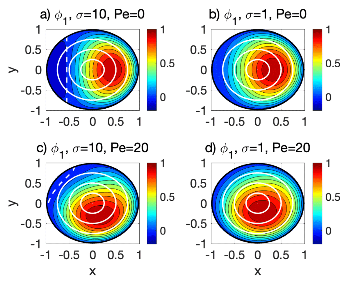
Figure 4
Upper-layer pressure φ1 (Eq. 46), which is proportional to the upper-layer geostrophic stream function, for two combinations of the parameter σ (Eq. 26) and the Peclet number. Here wa/wm = 4, implying that there is Ekman downwelling (upwelling) where x > –1/4 (). The amplitude of φ1 is normalised to be one at its maximum. The white lines show circles () that coincide with the depth contours, and dashed white lines show the zero contour of φ1.
To qualitatively measure the alignment between the upper-layer flow and the bottom topography we use the cosine of the angle between the flow and the depth contours defined by Eq. 1. Figure 5 shows the area-mean of |cos(α)| as a function of the Peclet number for the flow defined by Eq. (46) for three different values of σ and for two cases of wind-forcing asymmetries: wa/wm = 4 and wa/wm = 8. As expected, the alignment between the flow and the topography increases with the Peclet number but decreases with increasing values of σ. This is because the contribution of the asymmetric component H1a to upper-layer flow increases with σ as the flow becomes more surface intensified (see Eq. 46). Stronger wind-forcing asymmetry, measured by wa/wm, decreases the topographic alignment. For the present asymmetric wind-forcing (Eq. 42), the alignment approaches a minimum of when wa/wm becomes large for non zero values of σ. In this limit the upper-layer flow (φ1) is proportional to H1a. Notably for large values of Pe, the upper-layer flow becomes highly aligned with the depth contours, implying that .
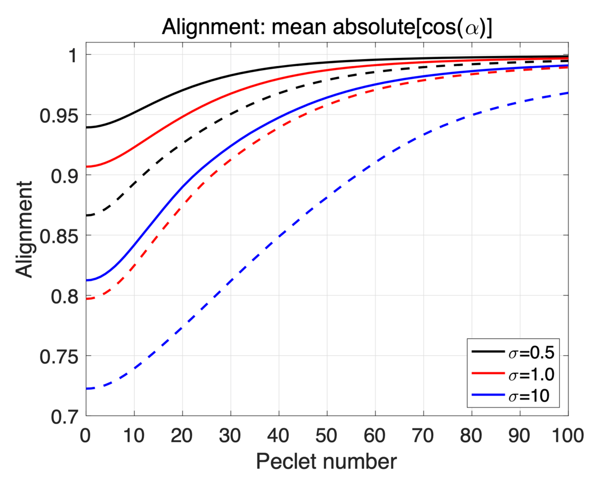
Figure 5
Alignment of the upper layer flow with the bottom topography as a function of the Peclet number for the flow field given by Eq. (46): see Figure 4. The topographic alignment is defined as the area mean of |cos(α)| (Eq. 1); perfect alignment corresponds to 1. Black, red, and blue lines correspond to σ = 0.5, σ = 1, and σ = 10, respectively. Solid (dashed) lines correspond to a wind forcing asymmetry – measured by wa/wm – of 4 (8). For this flow field the alignment for Pe = 0 and large values of σ approaches ≈ 0.8 when wa/wm = 4 and ≈ 0.7 when wa/wm = 8. If α – the angle between the isobaths and upper-layer flow – is randomly distributed in a domain then the area average of |cos(α)| is 2/π ≈ 0.6.
Figure 6 shows the topographic alignment of the upper-layer flow as function of the Peclet number and the parameter σ, for the flow defined by Eq. (46) with wa/wm = 4. When σ becomes small the flow becomes nearly barotropic and aligned with the topography. In this limit the alignment is weakly dependent on the Peclet number. The dependence of the alignment on σ is strongest when the Peclet number is small. The qualitative features of Figure 6 are similar to those for other values of wa/wm (not shown). The detailed features of Figure 6, however, can be expected to change slightly with the specific spatial form of the asymmetric forcing (Eq. 42).
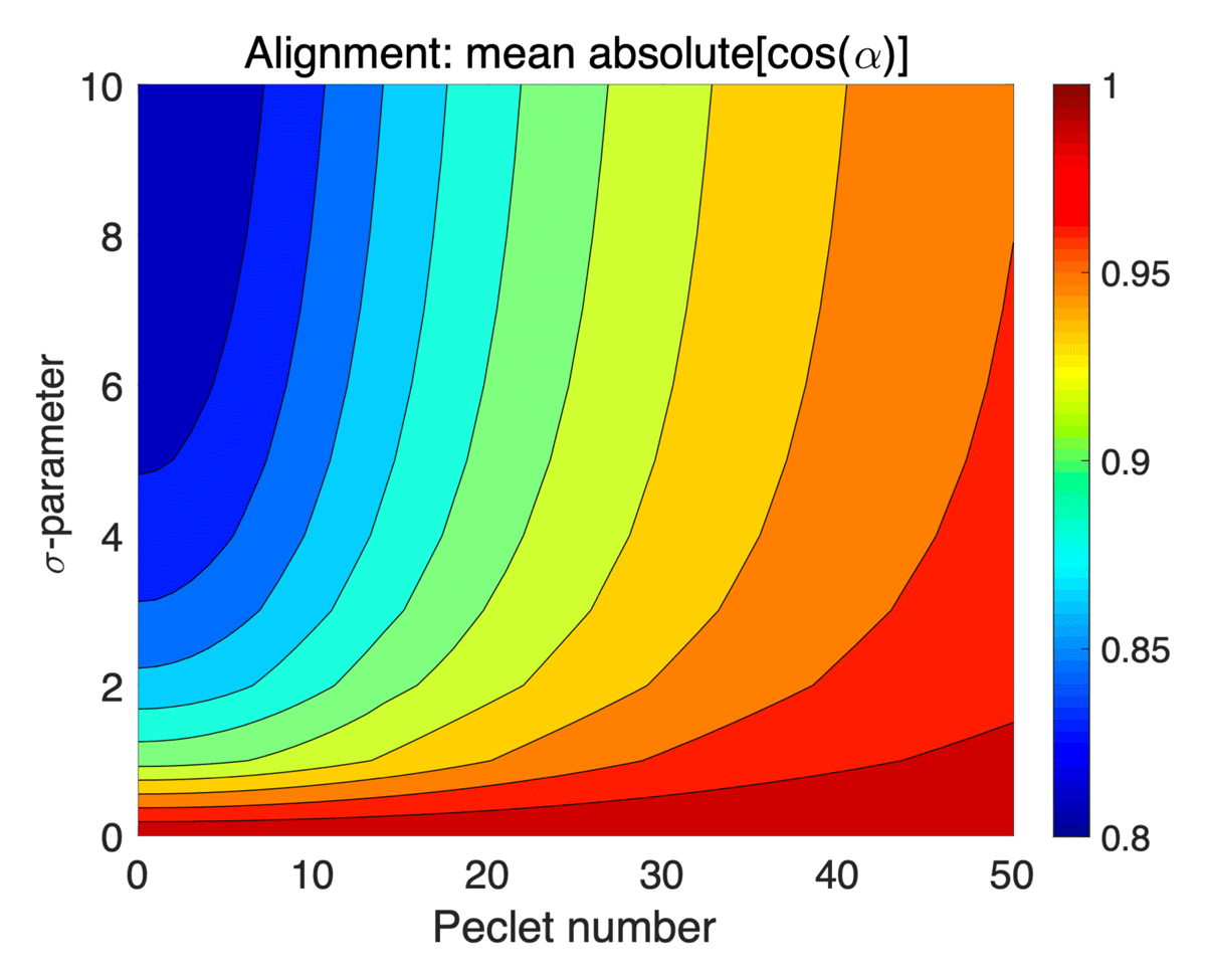
Figure 6
Topographic alignment of the upper layer flow as a function of the Peclet number and the parameter σ. The flow is given by Eq. (46) with wa/wm = 4. In this case the alignment for Pe = 0 becomes ≈ 0.8 for large values of σ, corresponding to a strongly baroclinic flow. When σ approaches zero the flow becomes barotropic and fully aligned with the topography.
We emphasise that the bathymetry in the real Beaufort Gyre, embedded in the Canada Basin, is complex (see e.g., Figure 1 and Timmermans and Marshall, 2020). Thus, the circular basin geometry used here is an extreme idealisation. Further, only depth contours deeper than around 2700 m close themselves locally in the Canada Basin, implying that shallower depth contours extend in the Arctic Ocean beyond the conventional geographical definition of the Canada Basin (Jakobsson, 2002). These features should be kept in mind when comparing our model results with the real Beaufort Gyre. Nevertheless, the present idealised model solutions should give some qualitative indications of how the real near-surface flow in Beaufort Gyre is influenced by the bathymetry via the Peclet number and the parameter σ (see Figures 5, 6). Further, Figure 4 suggests that the surface height maximum (proportional to φ1) should, for increasing Pe and decreasing σ, be shifted away from the maximum in downward Ekman pumping (located at x = 1 in Figure 4) and towards the ‘gyre centre’ which in the present model context would correspond to the location of the maximum basin depth in a non-circular basin. Observational estimates of the surface Ekman pumping and the surface height field in the Beaufort Gyre (see e.g., Figures 4 and 5 in Timmermans and Toole, 2023) suggest some degree of topographic influence of surface Beaufort Gyre flow on large scales, but also indicate local regions of significant cross isobath flow.
4.3 Norwegian Sea example: boundary forced asymmetries
We go on to consider a different situation in which advection of the upper-layer thickness by the lower-layer velocity can affect the bathymetric alignment of the upper-layer flow. Specifically, we consider a highly simplified model of the flow in a region with locally closed depth contours in the Norwegian Sea (see Figure 9) which again is idealised as a circular basin. In this example we take the upper layer to represent the Atlantic Water in the eastern Nordic Seas (Hansen and Østerhus, 2000). We assume that the flow is driven by local surface Ekman pumping, due to cyclonic wind forcing, as well as large-scale atmospheric-ocean interactions that drive a general northward flow of Atlantic Water through the domain in the upper layer (Walin et al., 2004; Spall, 2010). For the sake of simplicity, however, the Atlantic flow is here imposed as a boundary condition on an outer depth contour in the ‘gyre’. Thus, the ‘gyre boundary’ is taken to be a closed depth contour at the edge of a local basin in this case. We specify the inflow as well as the outflow in the upper layer on the ‘gyre boundary’ which is a fairly drastic simplification since the distribution of the outflow is likely to be affected by the locally wind-forced flow. However, this simplification allows analytical solutions that should illuminate aspects of the dynamics. As wind forcing we use a constant upward Ekman velocity in the gyre, associated with the isobath-following flow specified by Eqs. (38, 40, 41).
We consider a constant northward Atlantic Water flow, with the velocity vA, in the upper layer through the domain, which is imposed as a boundary condition at the gyre boundary (see Figure 7a). Note that Atlantic Water is now assumed to flow in the upper layer across the depth contours at the ‘gyre boundary’ causing φ1 to vary along the boundary, whereas in the Beaufort Gyre example we assume zero upper-layer flow at the gyre boundary (i.e. φ1 is taken to be constant). The associated H1 field is obtained as a solution to the homogeneous advection-diffusion equation (Eq. 35) and it is denoted H1A: see Eq. (A29). The amplitude of H1A is set by vA and its shape depends on the Peclet number: Pe = vGLG/K, where vG is the wind-forced lower layer flow (Eq. 39). The field φ1 is given as the sum of the isobath-following contribution (Eq. 41) and the contribution due to H1A; the non-dimensional φ1 then takes the form
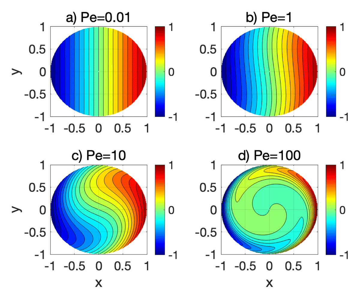
Figure 7
Solutions of upper-layer thickness H1A(x,y) forced by an imposed gradient at the gyre boundary (r = 1) where H1A = cos(θ) = x: see Eq. (A22). The solutions depict how a northward ‘Atlantic Water’ flow in the upper layer is affected by a cyclonic isobath-following flow that is forced by wind-stress over the gyre. For large vales of the Peclet number the flow becomes confined to boundary layers with a thickness on the order of Pe–1/2 (see Eq. A24). Note that since the upper-layer thickness is only advected by the lower layer velocity the shape of H1A(x,y) depends solely on the Peclet number based on the lower layer: Pe = vGLG/K (Eq. 39).
Figure 7 shows the asymmetric upper-layer thickness solution H1A (Eq. A29). In the absence of local cyclonic wind forcing v2 and Pe are zero. In this case the homogeneous solution H1A with Pe = 0 gives the whole field, which is a constant northward flow associated with an east–west gradient in H1A. When the wind forcing is increased H1A is distorted by the cyclonic flow. For very high Pe the variations of H1A become confined to thin layers at the gyre boundary and H1A becomes nearly constant in the interior gyre.
Figure 8 shows φ1 given by Eq. (47) for increasing values of vA/vG. Here we take Pe = 20 and σ = 0.5, values that roughly characterise the Norwegian Sea. Further, taking observed northward Atlantic Water velocities, which are in the range between 0.05 and 0.15 m s–1 (Hansen and Østerhus, 2000), we estimate that vA/vG is on the order of unity. When vA/vG is increased the upper-layer flow crosses the depth contours to an increasing degree but the lower-layer flow remains, by design, aligned with the depth contours. Further, the lowest value of φ1 in the gyre, which is at the gyre centre when vA/vG = 0, becomes displaced towards the south–west when vA/vG increases.
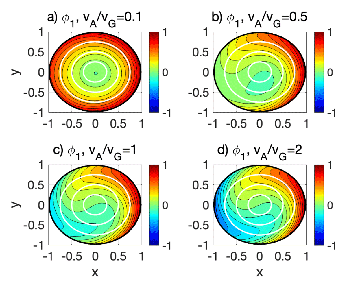
Figure 8
Solutions of upper-layer dynamic pressure φ1 forced by an imposed boundary northward flow of Atlantic Water and a uniform Ekman surface velocity (wE > 0): see Eq. (41). For all solutions, Pe = 20 and σ = 0.5. The panels shows different ratios of the imposed Atlantic Water velocity vA and the lower-layer gyre velocity vG: see Eq. (38). The solutions are normalised to range between –1 and +1.
Figure 9 shows the observed time-mean dynamic surface height in the eastern Nordic Seas. The dynamic height reveals a general northward flow of surface waters in the eastern Norwegian Sea and in the Lofoten Basin. In the Norwegian Sea there is also a tendency of a cyclonic circulation of the surface flow which has some qualitative similarities with the model flow fields shown in Figure 8b–c. For instance, the minimum surface pressure is displaced south–west of the deepest part (‘centre’) of the gyre.
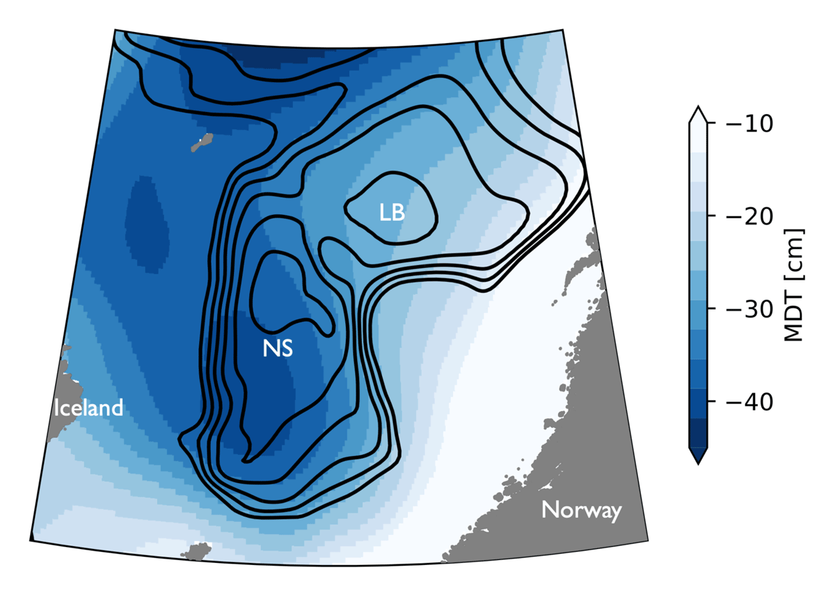
Figure 9
Time-mean dynamic surface height, based on satellite altimetry (Mulet et al., 2021), in the Norwegian Sea (NS) and the Lofoten Basin (LB). The dynamic height is proportional to the upper-layer dynamic pressure φ1 in the model. The black lines show depth contours. Figure 8 shows model solutions representing an idealised Norwegian Sea case.
5 Discussion
The present study was motivated by observations showing that the surface flow in the Arctic Ocean tends to be aligned with the bathymetry (see Jakobsen et al., 2003; Koszalka et al., 2011; Armitage et al., 2017, and Figure 1). To examine possible underlying mechanisms we developed and analysed a two-layer model. According to our analyses a key factor for the bathymetric alignment is the presence of closed depth contours which causes net surface wind stress to drive relatively strong near-bottom flows along the depth contours (Nøst and Isachsen, 2003; Aaboe and Nøst, 2008). This acts to suppress buoyancy variations (corresponding to variations in upper-layer thickness in the model) along the depth contours that are forced by variations in surface Ekman pumping and air–sea buoyancy fluxes and mixing; see Eq. (15). The observed tendency of upper-ocean topographic steering suggests that the flow is characterised by a relatively large Peclet number, implying that advection is more important than eddy diffusion in shaping the upper-layer thickness. In addition, the weak stratification in the Arctic Ocean makes the thermal wind velocity relatively small, yielding a fairly barotropic flow; see Eq. (26).
Figure 1, based on satellite altimetry, reveals a high degree of topographic surface flow alignment also in the Canada Basin where the surface currents and the surface wind stress are mainly anticyclonic (Timmermans and Marshall, 2020; Timmermans and Toole, 2023). This is broadly consistent with the present model and that of Nøst and Isachsen (2003), which are both linear and predict a generally anticyclonic deep flow in the Canada Basin that could extend through the water column, structuring the upper-ocean circulation to preferentially following the bathymetry. One caveat, however, is that standing topographic waves can emerge in an anticyclonic mean flow (with shallow water to the left). If this occurs topographic form stresses develop that add to the frictional bottom stress, an effect that can strongly reduce the strength of the near-bottom mean flow (Johnson and Bryden, 1989; Nøst et al., 2008; Constantinou and Young, 2017; Bai et al., 2021). In the context of the present model one can envision that form stresses result in a higher effective frictional bottom stress for anticyclonic flows – i.e. a higher value of the friction parameter R – than for cyclonic flows. Notably, increasing the effective R value will have a twofold effect on topographic steering of the upper-ocean flow: this increases σ and decreases the Peclet number (see Eqs. 20,29). Both effects yield a more baroclinic flow with reduced topographic influence of the upper ocean. However, the limited observations of the deep flows in the Canada Basin (see e.g. Aaboe and Nøst, 2008) make it difficult to decide if the deep currents are too weak to topographically steer upper-ocean flow in this part of the Arctic Ocean.
We also presented a ‘Norwegian Sea’ model case to examine how isobath-following near-bottom flows interact with a general northward flow of ‘Atlantic Water’ in the upper ocean (Figure 8). Despite that the model is highly idealised it captures some qualitative features of the surface flow in the Norwegian Sea. Figure 9 shows that the observed minimum surface pressure is displaced south-west of the deepest part (‘centre’) of the gyre and also hints a slight cyclonic rotation of the surface pressure field. These features are in broad agreement with the idealised model.
We underline that the present model includes a representation of the effect of mesoscale eddies on only the stratification (i.e., eddy fluxes of planetary potential vorticity, taken to diffuse H1). This model representation implies that the integrated wind stress input along an isobath is balanced by the integrated bottom stress on the same isobath. However, the model neglects effects of mesoscale eddies on the relative vorticity fluxes, or relatedly eddy momentum fluxes (Reynolds stresses), which can redistribute the surface wind stress input horizontally, across depth contours. Modelling studies suggest that cross-isobath eddy-induced momentum fluxes can affect the time-mean flow distribution along the continental slope in the Beaufort Gyre (Wang and Stewart, 2018; Manucharyan and Isachsen, 2019; Nummelin and Isachsen, 2024). In the eddy-rich Lofoten Basin, modelling also suggests that the structure of the time-mean flow is influenced by horizontal eddy vorticity fluxes (see e.g. Spall, 2010; Trodahl et al., 2020).
Finally, we underscore that in the present model it is only the lower-layer flow that advects and interacts with the upper-layer thickness, related to the buoyancy field in a continuous representation. If the time-mean lower-layer flow is negligible then the upper-layer flow is blind to the topography in our model. In reality, however, time-dependent motions associated with baroclinic eddies and flows forced by passing storms generally sense the bottom topography. Accordingly, the aggregated effect of the time-dependent flow on the buoyancy distribution may carry an imprint of the bottom topography. Indeed, analyses of floats and ocean-circulation experiments, as well as theoretical considerations, show that the effective diffusivity is significantly weaker across depth (or f/H) contours than along them (e.g. LaCasce, 2000; Isachsen, 2015; Wei et al., 2022; Nummelin and Isachsen, 2024; Sterl et al., 2024). This is a potentially important additional mechanism for topographic steering of the time-mean surface flow which could be represented in the present model by introducing an anisotropic topographic-slope dependent thickness diffusion.
Appendices
Appendix: Mathematical Relationships
The topographically-steered limit: integral relations
We will here examine how the flow is organised when the parameters Pe–1 and ε are small. In this limit the flow follows the depth contours, to the lowest order, in both layers which are thus equivalently barotropic. Here, the flow field on closed depth contours can be determined from two integral relations, using the ideas presented by Nøst and Isachsen (2003).
Lower layer
The constraint that the lower layer follows the H contours (Eq. 30) implies that φ2 is a function of H alone, i.e. φ2 = φ2(H). Therefore, the lower-layer velocity can be written as
or alternatively
Here we have introduced
where and are the mean lower-layer velocity and slope on the closed depth contour C(H), respectively. As defined here, for cyclonic flow with shallow water to the right.
To determine we use the integral relation Eq. (18) and insert Eq. (A2) that applies on closed H-contours. After a few algebraic steps (Nøst and Isachsen, 2003) we obtain
where the right-hand side equals the mean along-contour wind stress divided by the bottom friction parameter R. This is the two-layer, f-plane version of the expression for the bottom velocity derived by Nøst and Isachsen (2003).
Upper layer
We can also derive an integral relation from Eq. (15) that determines the upper-layer thickness H1 in the limit where and ε are small. In this limit also the upper-layer flow is aligned with the depth contours, i.e. , and from Eq. (4) it follows that also . We write the upper layer velocity as
where
and we have used Eq. (4) to get the expression on the far right-hand side.
To determine we consider the steady-state version of Eq. (15) and integrate it over an area A(H) enclosed by a C(H) contour. By applying Gauss’ and Stokes’ theorems we obtain
where dA is the area element, and s are unit vector normal to and along C, respectively, and ds is the length element along C. The first term vanishes because u2 · n is zero: the lower-layer flow is aligned with the H contours. Using that H1 = H1(H), Eq. (A7) can be rewritten as
By dividing this expression with the length of the contour C and multiplying with we obtain
where we have introduced
By using Eqs. (A4,A6,A9) we obtain the following expression for :
where we used the definition of σ (Eq. 26). The term is associated with vertical volume transfer between the layers: transfer from the upper to the lower layer yields cyclonic upper layer circulation.
Analytical solutions for circular basins
Here we will derive analytical solutions for H1 in a basin with circular depth contours for simple but relevant asymmetric wind forcing fields. Note that no restrictions on the Peclet number are made here. The radial coordinate is non-dimensionalised with the gyre radius LG. Specifically, we will consider the case where the lower-layer velocity is solid body rotation (v2 = r) corresponding to a constant area-mean wE: see Eq. (38). In this case, the non-dimensional version of the advective–diffusive equation (Eq. 35) takes the form
Here, and the gyre velocity scale vG is defined in Eq. (39).
Solutions forced by asymmetric w′E
We seek a solution for the upper-layer thickness forced by which we label H1a. We make the ansatz
where m is an integer and Jm the Bessel function of order m. This ansatz is an eigen function of the Laplace operator in cylinder coordinates: (Arfken, 1985). At the gyre boundary r = 1 we assume solid coastal boundaries and zero normal flow which is satisfied if k is selected such that Jm(k) = 0. This allows the forcing and H1a to be expressed as sums of the form (Arfken, 1985)
Here, kmn is the n:th root of Jm, and amn and bmn constants. The terms in the series are linearly independent and orthogonal. This means that by inserting Eqs. (A14,A15) in Eq. (A12) we obtain
This relates bmn to amn, where amn is determined by shape of the Ekman forcing. After a few algebraic steps the solution of H1a can be written as
where
Here ϕ is a phase factor: ϕ > 0 (ϕ < 0) for cyclonic (anticyclonic) lower lower-layer flow.
Specifically, we seek a solutions to the asymmetric wind forcing
for which m = 1. In this case there is a single term in the sum over m in Eq. (A17) which simplifies to
where kn is the n:th zero of J1. The coefficient bn is obtained by expanding r in J1-series (Arfken, 1985); the result is
Boundary forced solutions
Motivated by dynamics in the Norwegian Sea, we here seek solutions with that are forced by specifying H1 on the domain boundary r = 1. We make the ansatz
which when inserted in Eq. (A12) yields the following equation for
By introducing the complex coordinate
Eq. (A23) transforms to
with solutions that are modified Bessel functions Im(z) (Arfken, 1985). The solution is complex but two real and linearly independent solutions can be extracted from it. By defining the real and imaginary parts
where Cm and Dm are real, the two solutions can be written as
This implies that the general H1A solution can be written as
where am and bm are constants determined by the boundary condition on H1A at r = 1.
We consider a solution for the boundary condition
for which m = 1. In this case the series in Eq. (A29) yields a single term, i.e. . Straightforward calculations shows that
Acknowledgements
We thank Ole Anders Nøst and Gösta Walin for some insightful comments at an early stage when J. Nilsson and P.E. Isachsen started to develop a ‘two-layer Arctic Ocean’ model.
Funding Information
This research has been supported by the Swedish Research Council (grant no. 2020-05076), the Swedish National Space Agency (grant no. 2020-00171) and the Research Council of Norway (TopArctic: grant no. 314826).
Competing Interests
The authors have no competing interests to declare.
Author Contributions
J. Nilsson and P.E. Isachsen conceived the ideas of how a two-layer model could be used to merge existing theoretical concepts of Arctic Ocean dynamics. J. Nilsson and J.A. Kallmyr developed the mathematical solutions and J.A. Kallmyr did the observational analyses. All authors contributed to the writing of the manuscript.