
1. Introduction
Aquatic ecosystems receive multiple pollutants from diffuse and point sources and act as sinks for various pollutants. Any type of river water contamination, whether direct or indirect, could be very dangerous to people’s health because they are the final consumers. Water is necessary for the metabolism of cells and correct functioning; thus, it can cause a variety of disorders in humans (Alam et al., 2017). According to Khanna and Ishaq (2013), dangerous wastewater that is discharged into rivers is a major global problem because it has a negative effect on aquatic life. The quality of water reflects environmental disturbances in their surrounding regions through the water quality (Khan et al., 2022). Due to climate change, increasing urbanization, food demand, and unrestrained use of natural resources, almost 40% of the world’s population is currently experiencing water scarcity (Scanlon et al., 2023). Recently observed is a significant increase in the release of polluted wastewater into the environment due to increased urbanization, industrialization, agricultural activity, geothermal water release, and olive wastewater discharge, particularly in places where olives are grown (Wijerathna et al., 2023). According to the previous reports, approximately 80% of the diseases reported in developing countries are caused by water pollution, since approximately 4 million deaths and an estimated 2.5 billion illnesses are reported from water pollution (Ahmed et al., 2019; Rafiee, 2018). Notable diseases in Pakistan are observed, including diarrhea, typhoid, gastroenteritis, cryptosporidium infections, hepatitis, and giardiasis intestinal worms (Zhao et al., 2024; Noureen et al., 2022), which affect the country’s GDP in the range of 0.6 to 1.44% (Jabbar, 2020) and become an urgent and vital issue in Pakistan. Since water contamination affects different regions and countries (Sharma et al., 2022), almost a billion individuals have faces lake access to safe drinking water, resulting in two million deaths occurring annually because of water contamination, poor sanitation, and unhygienic conditions (Kumar et al., 2022).
The presence of nitrates and heavy metals in water captured the attention of many water quality researchers worldwide (Unigwe & Egbueri, 2023). Water covers approximately 70% of the Earth’s surface and plays an important role in human survival, such as being used for domestic, agriculture, and industrial activities (Khan et al., 2023). However, water quality is reduced due to heavy metal contamination (Balali-Mood et al., 2021; Rafiee, 2018; Tchounwou et al., 2012) and causes cancer in the kidneys, blood, and cardiovascular and nervous systems (Firisa, 2023; Genchi et al., 2020; Tchounwou et al., 2019; Ulapane et al., 2023). Lead exposure damages the nervous system and kidney function, which is especially hazardous to children and pregnant women (Chan & Qi, 2003; Ray et al., 2009; de Jesús Rubio et al., 2023; Yu et al., 2017). Furthermore, climate change has made it difficult to get fresh water in areas already affected by pollution through increasing temperatures, frequent floods, and drought persistence (Li et al., 2023; Ling et al., 2024). After the industrial revolution and the scientific growth of humans, additional environmental contaminants entered water, soil, and air, as well as increased entrance of these compounds into plants, particularly vegetables, through water. Continuous growth in the human population spread urbanization, industrialization work, technical improvement, and growth in agriculture, resulting in a lack of natural freshwater bodies, including lakes, wetlands, and rivers (Ibrahim and Nafi’u, 2017). It is a global issue, affecting both the environment and public health (Buckley & Casson, 2003; Stephenson, 1993). Agricultural products contaminated with heavy metals reduce their quality while also posing a major threat to human health. Some synthetic organic dyes could cause health and environmental issues because they contain toxic components (Chen et al., 2022). Therefore, environmental considerations are critical, and heavy metals, including copper, zinc, and cobalt, are critical for many biological systems.
Monitoring water quality parameters according to relevant standards is essential, but the traditional approach to water quality parameter monitoring is limited due to its lack of expansiveness and technical difficulties (Mostofi, 2018; Zhu et al., 2022). However, by using machine learning algorithms, the complexity of non-linear relationships could be easily dealt with, which can handle the underlying discovery mechanisms (Ray, 2019; Li et al., 2022). In recent years, many researchers have believed in the advancement of machine learning that highly dimensioned data can be captured successfully and evaluate the complex and large scale of water quality requirements (Zhu et al., 2022). The Boruta algorithm was employed to find significant influential factors and improve the model performance associated with water quality classification (Jamei et al., 2022). Simply put, the model’s efficiency can be elevated by identifying the valuable factors and eliminating the unnecessary factors corresponding to the water quality classes.
In literature, various machine learning algorithms frequently employed for classification and regression, including the decision tree model (Saghebian et al., 2014; Sihag et al., 2021a), the k-nearest neighbor method (Naimi et al., 2022), the multiple perceptron neural network model (Abba et al., 2021; Juna et al., 2022), support vector machine model (Ehteram et al., 2021; Sakaa et al., 2022), the relevance vector machine model (Pham et al., 2021), the random forest model (Alnahit et al., 2022; Sihag et al., 2021b), the M5 three and random subspace model (Almohammed et al., 2022; Pande et al., 2023), and others (Maroufpoor et al., 2022) have been employed for estimating quantitative target variables (Dai et al., 2024; Hrnjica et al., 2021). Since we know that water quality is important factor for living, numerous researchers and environmental scientists have utilized various methods to monitor and classify it. It gives a complete evaluation of the methodology used for monitoring water quality classification based on the existing literature. Various traditional measurements have been used for water quality when the enumerator wants to collect data about the water quality assessment, like manual data collection from different locations, laboratory analysis, calculating the water quality index, and experimental work carried out on the critical parameters that affect water quality (Jayaraman et al., 2024; Wu et al., 2021). To calculate WQI, it involves the selection of water quality class categories and computing the sub-index, along with the aggregation function. All these calculations are crucial to calculating the WQI that affects the water quality class (Hipsey et al., 2020; Uddin et al., 2022). Zhang et al. (2022) explore the utilization of the ultraviolet spectroscopy and the CNN model for the monitoring of water quality. So, the standard normal and multiplicative correction methods have high accuracy in total organic carbon and total suspended solid parameters. In 2022, Zhang et al. introduced the AT-BILSTM model for forecasting watershed water quality. Li et al. (2020) used three deep learning models, including RNN, LSTM, and GRU, to estimate the dissolved oxygen concentration in the region’s fishing ponds. Furthermore, T^2-bsased principle component analysis could be affected by an outlier if there is an outlier in observation, and it gives an incorrect result in classification.
Therefore, many modifications have been developed to solve this problem. The hotelling T^2-based principle component analysis control chart and T^2 statistic were widely used for the detection of outliers. For classification problems, T^2 and Q-statistics have been frequently used (Eide and Westad, 2018; Li et al., 2018; Ruiz et al., 2004). However, due to the complexity and time consumption of a data-driven model, it might be an uncertain prediction (Bui et al., 2022). Moreover, the advancement of machine learning and deep learning has significantly impacted a vital role in water quality assessment and has fundamentally changed our prediction methods and understanding of environmental data. This research study focuses not just on assessing and predicting water quality class but also on identifying the harmful factors in the water and rivers in Khyber Pakhtunkhwa, Pakistan. To resolve water quality issues, various machine learning algorithms were employed, including the Boruta algorithm to overcome the complexity of the model, the decision tree model, the k-nearest neighbor method, the multilayer perceptron algorithm, the support vector machine, and the random forest algorithm. The aim of this study is to protect human health from harmful heavy metal contamination and serves as a significant guideline for water quality management and resource management in the Eastern Hindukush regions of Pakistan.
2. Methodology
2.1. Description of study and location
The present study examines and evaluates the water quality in various glacial Alpine lakes and glacier-fed rivers, including the Swat and Panjkora Rivers in Khyber Pakhtunkhwa, Pakistan. These glacial lakes have a critical role in maintaining the daily lives of approximately 10 million people by providing drinking water and are used for agriculture, electricity, and recreation purposes. Tourism plays a vital role in the economy of the northern areas of Pakistan but has negative impacts on the water quality of the Swat and Dir regions. (Muzamil, 2021). The interconnection of the Alpine glacial lakes with the studied rivers, surrounding landscapes, and floodplain areas highlights the significance of comprehensive management techniques to control and overcome pollution and protect these vital water resources. The dataset for this investigation was obtained from a previous study conducted by Khan et al. (2022), as shown in Figure 1 using ArcGIS. In this research study, 79 samples were collected from the Swat and Panjkora rivers. Swat is located in the northern mountain ranges. The temperate zone in the Swat region has elevations ranging from 500 to 6,500 meters above sea level (Qasim et al., 2011). Swat is located between 34 and 36 degrees north latitude and 71 and 73 degrees east longitude, with an area of 5,337 square kilometers. In Pakistan’s eastern Hindukush region, the Swat River is a major flood-prone area and travels 288 kilometers from the Seri Kalam Valley to Sardaryab Charsadda (Nasir et al., 2023). The Swat River starts in Kalam with the merging Ushu and Utror rivers and runs downstream through the valley for 160 kilometers to Chakdara. It covers more than 250 kilometers from Kalam to near Charsada. Numerous large and small tributaries join this river. Among them, the Panjkora River is 220 kilometers long and flows south through Dir Upper and Dir Lower districts until joining the Swat at Bosaq. It is situated at the intersection of Dir Lower, Bajaur Agency, and Malakand, and then continuously travels downstream as the Swat River. Additionally, the Panjkora River ultimately enters the Kabul River in the area of Charsadda.
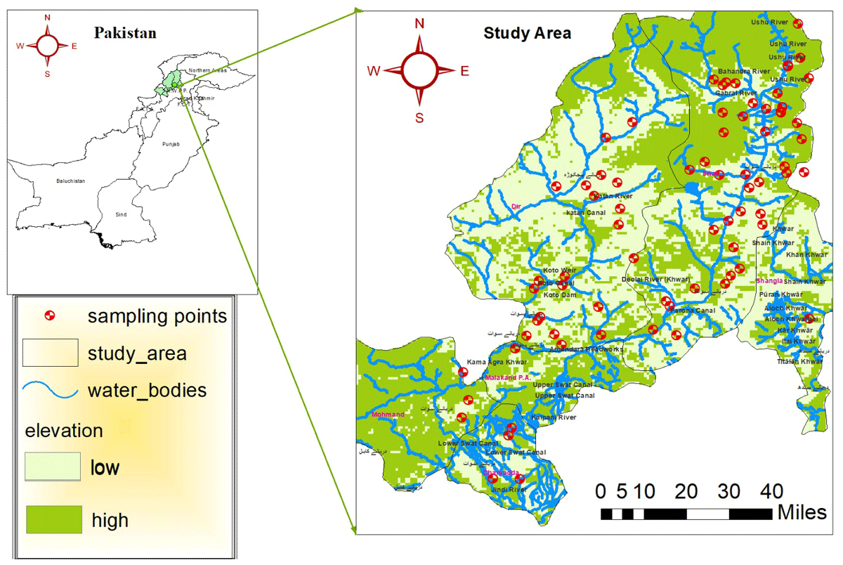
Figure 1
Location of the study area in Khyber Pakhtunkhwa, Pakistan.
2.2. Methods
The main stages in developing the classification of water classes are as follows. Before fitting the models, we use the Boruta technique to identify critical parameters related to water quality classes. To model water quality classification utilizing DT, KNN, MLP, SVM, and RF, we selected a collection of 79 water samples, with their respective quality classes acting as the model’s inputs and outputs. In this configuration, water quality parameters serve as the model’s input, while water quality classes are generated from the WQI during the models fitting in this research study. During models fitting for this study, 70% of the dataset was used for the training set, and the rest of the dataset was used for the testing dataset in order to generalize our result. Figure 2 provides a graphical representation of the various phases of the current investigation during this research. It starts with data collection and ends with the preprocessing of the data before calculating the WQI. The Boruta algorithm was applied to identify the significant factors for the water quality class. Furthermore, machine learning algorithms, including the decision trees model (DT), the multi-layer perceptron (MLP) algorithm, the k-nearest neighbors method (KNN), the support vector machines (SVM) model, and the random forest (RF) model, are used to develop water quality prediction.
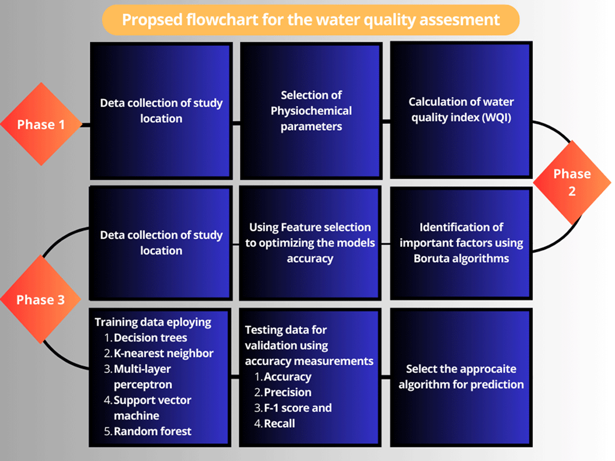
Figure 2
Flowchart of the applied process for the water quality classification.
2.3. Water quality index (WQI)
The main objective of water quality is to provide an overall assessment by considering various parameters and heavy metals and simplifying the difficulties as a standard method for evaluating the water quality in the world. The WQI was developed by Horton (1965) in the United States, and it was further modified by Brown et al. (1970). Recent studies have been extensively conducted for water quality assessment globally (Das et al., 2022; Kachroud et al., 2019; Udeshani et al., 2020). Furthermore, the weights were added in 2001 when computing WQI to determine the water quality class. For a detailed description, see Cude (2001). Over time, it was improved by different researchers (Hooshmand et al., 2011; Qasim et al., 2011; Raza et al., 2021; Sani et al., 2022; Uddin et al., 2021; Wali et al., 2020a; Wali et al., 2020b; Wali, et al., 2021; Wali et al., 2022). In this research study, the weighted arithmetic method was employed to calculate WQI because it is the most widely used method in both surface and groundwater studies (Călmuc et al., 2018; Tyagi et al., 2013). WQI was calculated for the river at the nine most used water quality parameters and screened for heavy metals such as cadmium (Cd in mg/L), chromium (Cr in mg/L), lead (Pb in mg/L), nickel (Ni in mg/L), iron (Fe in mg/L), arsenic (As in mg/L), power of hydrogen (Ph), electrical conductivity (Ec in µS/Cm), and total dissolved solids (TDS in mg/L). The weights are assigned to each physicochemical parameter of water according to their relative importance in determining water quality.
Computing WQI is given by the following formula:
Where
and
In equation (1), represents the ith parameter. In equation (2), is the weight of the ith parameter, heavy metals, and indicates the quality rating of the ith parameter of water. In equation (3), denotes the value of each parameter in the sample of water, while denotes the standard value of the ith parameter of water. In Table 1, the WQI is categorized (Khan et al., 2022; Tyagi et al., 2013).
2.4. Boruta technique
The Boruta algorithm is utilized as the water quality parameter selection in this research, and it can select optimal parameters conveying relevant information for model prediction. The Boruta method, proposed by Zhang et al. (2020), is employed here to achieve this goal. The Boruta algorithm is based on R programming, which employs the importance measure provided by the original algorithm. It is based on a random forest implementation that uses a single function to identify all of the important parameters in a dataset in relation to an outcome variable. The number of estimators is predefined in this research study as the Boruta algorithm in R-programming and allows an automated number of estimator selection rather than finding a possibly compact subset of the parameters of water and heavy metals in a dataset because it is applicable to all types of parameters. The Boruta algorithm was utilized with settings such as doTrace = 2 and maxRun = 500 to identify the minimal optimal parameters and heavy metals for fitting the models.
2.5. Decision tree (DT) model
The DT model is a key tool in the context of machine learning algorithms, depending on labeled training data to produce accurate predictions. It divides the dataset systematically into smaller subsets and performs tests at each node in the tree (Friedl and Brodley, 1997). A basic feature of decision trees is their frequent ability to segment the training set of the data and examine relevant attribute information and classification results. The primary goal is to build a decision tree that facilitates successful decision-making (Ren et al., 2022). Each route from the starting node to the leaf node in the DT model contains a set of rules, providing practical categorization rules that can be tested on real-world data. This hierarchical model uses an iterative process of categorizing the group of independent variables into homogeneous groups while highlighting essential characteristics at nodes from top to bottom (Hssina et al., 2014; Li et al., 2022). The Gini index is a crucial measure of inequality used in the DT model (Berndt et al., 2003; Ceriani and Verme, 2012). In the DT model, the Gini index helps in the selection of the most important parameter to split the data at each node, aiming to reduce impurity and increase homogeneity among the resulting subsets. Both the training and validation sets are used in the DT model to evaluate it. The DT model works similarly to a flowchart, as shown in Figure 3, based on the training data.
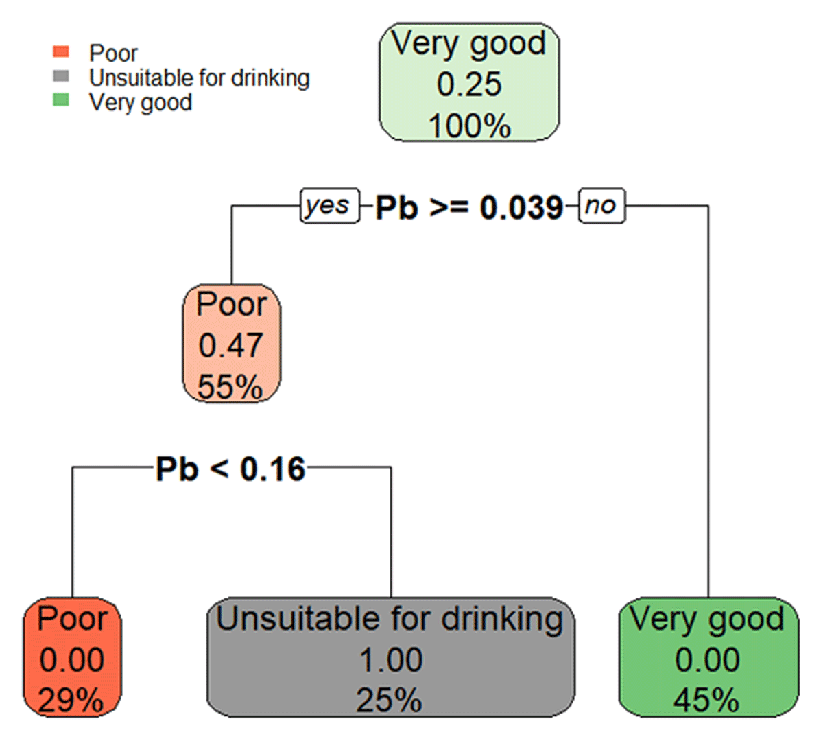
Figure 3
Decision tree visualization using the training set insight into model training.
2.6. K- nearest neighbor (KNN) method
Due to its popularity and robust performance, the KNN method is extensively used in data mining and machine learning applications, as observed in studies (Khamis, 2014; Wang et al., 2022; Zhang et al., 2017). Although famous for its simplicity and efficacy in classification, it has some drawbacks. Its efficiency is low, and it faces difficulties in k parameter selection. During a specific search, the KNN identifies the nearest data points from a provided training dataset. Once the k-nearest neighbor points are identified based on their distance from the search point, the algorithms employ a majority voting for the most major class and the rest for the minor class. In this research study, the KNN method was employed based on the training dataset, and then the model was trained with different values of k ranging from 1 to 10. Through this approach, the optimal value of k was determined to be 9 for this search. Furthermore, the model’s performance was evaluated using the rest of the dataset.
2.7. Multi- layer perception (MLP)
Neural networks, particularly the MLP model, are widely viewed as requiring less domain-specific expertise for optimal performance. This is due to their ability to iteratively and independently tune parameters (Aitkin and Foxall, 2003; Piramuthu et al., 1994). This feature dramatically reduces the amount of time and human input required, speeding the machine learning process. It is a traditional model of neural networks mostly employed for classification problems (Sharma et al., 2022). For the classification task, nodes in the input and output layers in the MLP model are based on the number of parameters and classes. Moreover, in the MLP model, additional configuring includes, the number of hidden layers, node allocation to each hidden layer, complete iterations, and also weights learning when using MLP-NN (Azad et al., 2022; Hrnjica et al., 2021). The input layer contains the prediction parameters that affected the prediction class, and the output layer derives the prediction based on those affected factors. In this article, we used an R “neuralnet” function after training the MLP-NN to determine the setup of neurons within the neural network’s hidden layers.
2.7.1 Proposed Architecture
The hidden parameter is used in R “neuralnet” functions with an activation function such as a logistic function. After training the MLP-NN to determine the setup of neurons within the neural network’s hidden layers, Should not be selected randomly as the number of hidden layers and neurons when fitting the MLP model. Using too many layers and neurons can cause overfitting of the model; similarly, using a smaller number of neurons and hidden layers might be cause underfitting of the MLP model. Therefore, deciding the number of hidden layers and neurons should be done carefully. Two hidden layers are optimal for prediction studies. In difficult problems, one or two hidden layers provide optimal results in classification, as suggested in the given article (Panchal et al., 2011). There are two hidden layers used here for modeling, as shown in Figure 4. In each layer, we used hidden layer = (9,9) based on the formula (2/3 multiplied by the size of the input layer) and then added the size of the output layer (Panchal et al., 2011).
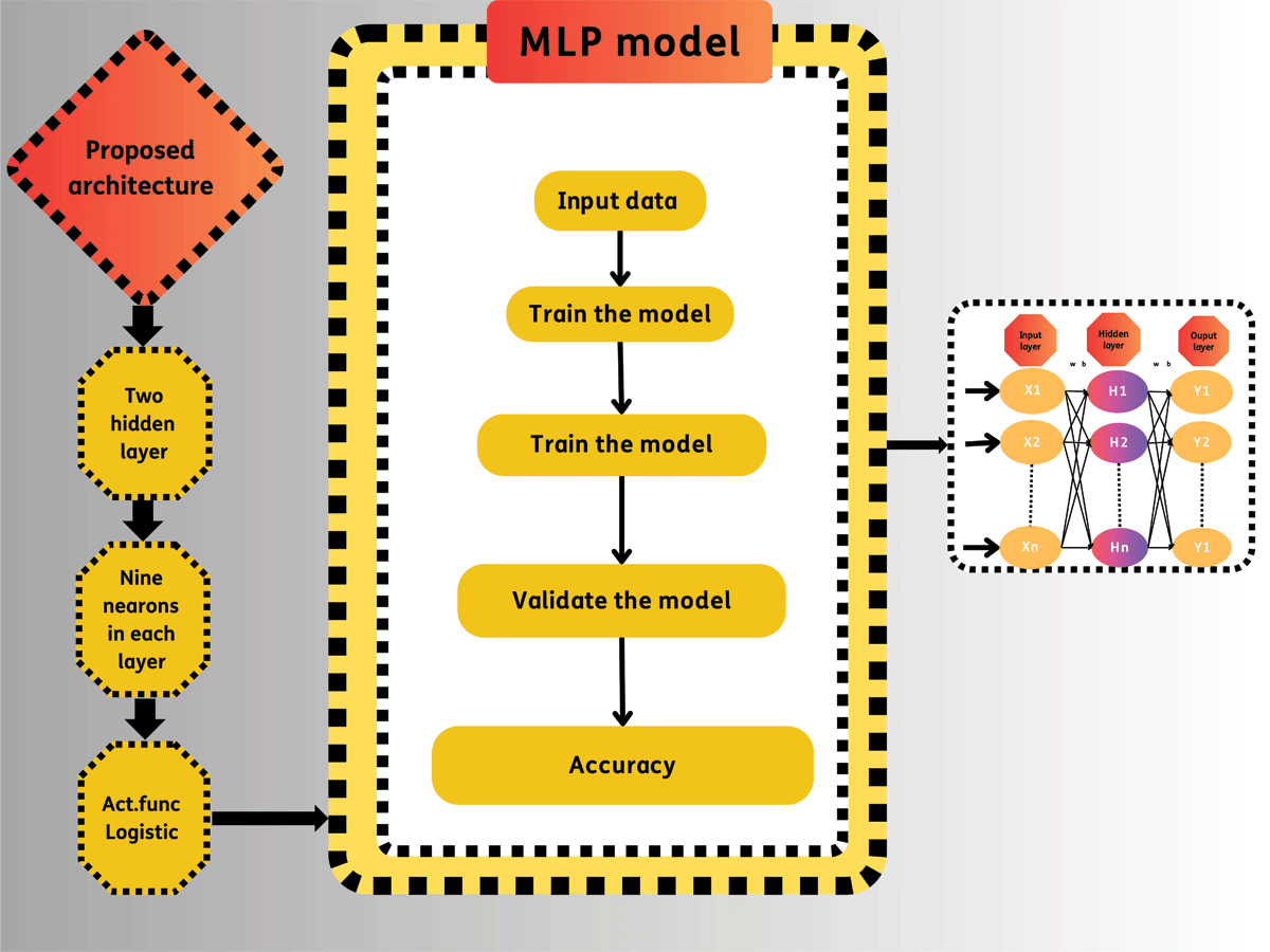
Figure 4
Multiple layer perceptron for water quality classification.
2.8. Support vector machine (SVM)
We used the SVM model with varied settings in our research. To build the SVM model in this research, e1071 package was used to implement the model. Different kernel functions were examined to determine how they affected the model’s performance, like linear, radial, and polynomial kernels. The SVM is a strong tool for categorizing and predicting (Patle and Chouhan, 2013), and we wanted to identify the optimal parameters and kernels for our particular case. This extensive method emphasizes the significance of the SVM model prediction and model performance. The key challenge in the classification process is determining the hyperplane that separates these classes, and this hyperplane is dependent on the maximum margin (Banerjee and Mondal, 2023). The SVM can handle a variety of optimization problems, including regression and data classification (Gunn, 1998). To distinguish between two categories, which can also hold the data if they have more than two categories, a hyperplane must be identified to partition the data points into two classes. For a more detailed description of the SVM model, see Baccour et al. (2022).
2.9. Random forest (RF) model
RF is a popular machine learning model widely used for both classification problems and regression problems, and it was developed by Breiman (2001) with a set of decision trees with controlled variation. The RF model is employed for both classification and regression analysis but is commonly used for classification (Jakhar et al., 2023; Li et al., 2022). It constructs several decision trees from the input data. Each decision tree generates a prediction output from each of the decision trees separately. The final prediction is determined by aggregating votes from different decision trees to select the best prediction (Pandimurugan et al., 2022). The number of decision trees in the RF model increases from the input data, and the precision of the RF model also increases, resulting in an effective model prediction (Breiman, 2001; Strobl et al., 2009). The accuracy of the RF algorithm mainly depends on the individual tree classifiers and the relationship between the classifiers (Amit et al., 1997; Galiano et al., 2012). Involving two main parameters, one is the number of trees, which is denoted by (ntree) in R language, and the second is (mtry), which is the number of variables. To optimize the model, we used various numbers of trees and numbers of variables at each node in the RF model.
2.10. Model performance evaluations
2.10.1. Accuracy
Accuracy serves as a metric that measures the overall correctness of the model. It is calculated by the number of correct predictions, classincluding the sum of the true positives and true negatives, and then divided by the total number of predictions class. In Equation (4), it is derived using TP, where TP is true positive, similarly TN (true negative), FP (false positive), and FN (false negative) (Alqahtani et al., 2022; Anđelić et al., 2023; Koranga et al., 2022).
2.10.2. Precision (Positive predictive value)
Precision is a measure of a model’s accuracy in making good predictions when we are fitting various models. In equation (5), we devide the total number of positive predictions class by the sum of true positive and false positive predictions class. False positive predictions will be rare when precision is high (Armah et al., 2014; Miao & Zhu, 2022).
2.10.3. Recall (True positive rate)
According to the following, in equation (6), Recall is defined as the ratio of true positives (TP) to the sum of true positives and false negatives (FN) in the model. It captures all actual positive classes in the model, and it is also called sensitivity. A greater recall value suggests that the model was successful in identifying most positive cases (Armah et al., 2014; Koranga et al., 2022; Miao & Zhu, 2022).
2.10.4. F1-score
The F1 score provides the model performance that combines precision and recall statistics. According to the following in equation (7), using the harmonic mean of precision (also defined in equation (6)). The range of the F1 score is from 0 to 1. A lower F1 value indicates that the model performance, in terms of precision and recall, is poor fitting, and a high value of the F1 score indicates that the model performance is better as compared to other models.
3. Results and Discussion
Water is necessary for many human activities, including agriculture, residential use, recreation, and industry. Unfortunately, agricultural and human activities frequently pollute water sources, posing a severe danger to water quality. Water quality is traditionally calculated using water quality criteria obtained through a time-consuming laboratory examination. For water quality prediction, various machine learning algorithms are used for estimating and predicting WQI based on the nine parameters and heavy metals. Except Ec in µS/Cm and Ph in number, all the parameters and heavy metals are represented using a mg/L scale. The findings of the study classified the water samples into three distinct categories: very good, poor, and unsuitable for drinking. According to the WQI classification scale proposed by Brown et al. (1970), most samples of the dataset fell into ‘Very good (51.9%)’, and the other two classes (24.05%) were identified as the same, unfortunately, as shown in Figure 5. All the summary results presented in Table 2 are in the units of mg/L and uS/Cm. Cadmium (Cd) levels are within an acceptable range, with a standard value of 0.05; mean, minimum, and maximum values are 0.04, 0.01, and 0.07, respectively, and showed a low standard deviation of 0.01. However, chromium (Cr) varies significantly because it exceeds the normal range of 0.03. The average concentration is 0.05 mg/L, with a wide range of 0 to 0.18 mg/L and a standard deviation of 0.04 mg/L. Lead (Pb) levels are of great concern because they surpass the standard threshold of 0.01 mg/L based on the World Health Organization’s (WHO) standard value. The mean concentration of 0.19 mg/L, with a wide range of 0.01 mg/L to 0.91 mg/L, exhibits a high standard deviation of 0.29 mg/L. Nickel (Ni) and iron (Fe) levels are adequate; however, arsenic (As) levels are routinely recorded at 0 mg/L, indicating probable measurement problems. The Ph is within the acceptable range of 6.5–8.5, with a mean of 7.74. Electrical conductivity (Ec) and Total Dissolved Solids (TDS) both deviate significantly from the acceptable standard values of 400 S/Cm and 500 mg/L, suggesting excessive levels. The average Ec is 107.14 S/Cm, while the average TDS is 53.98 mg/L.
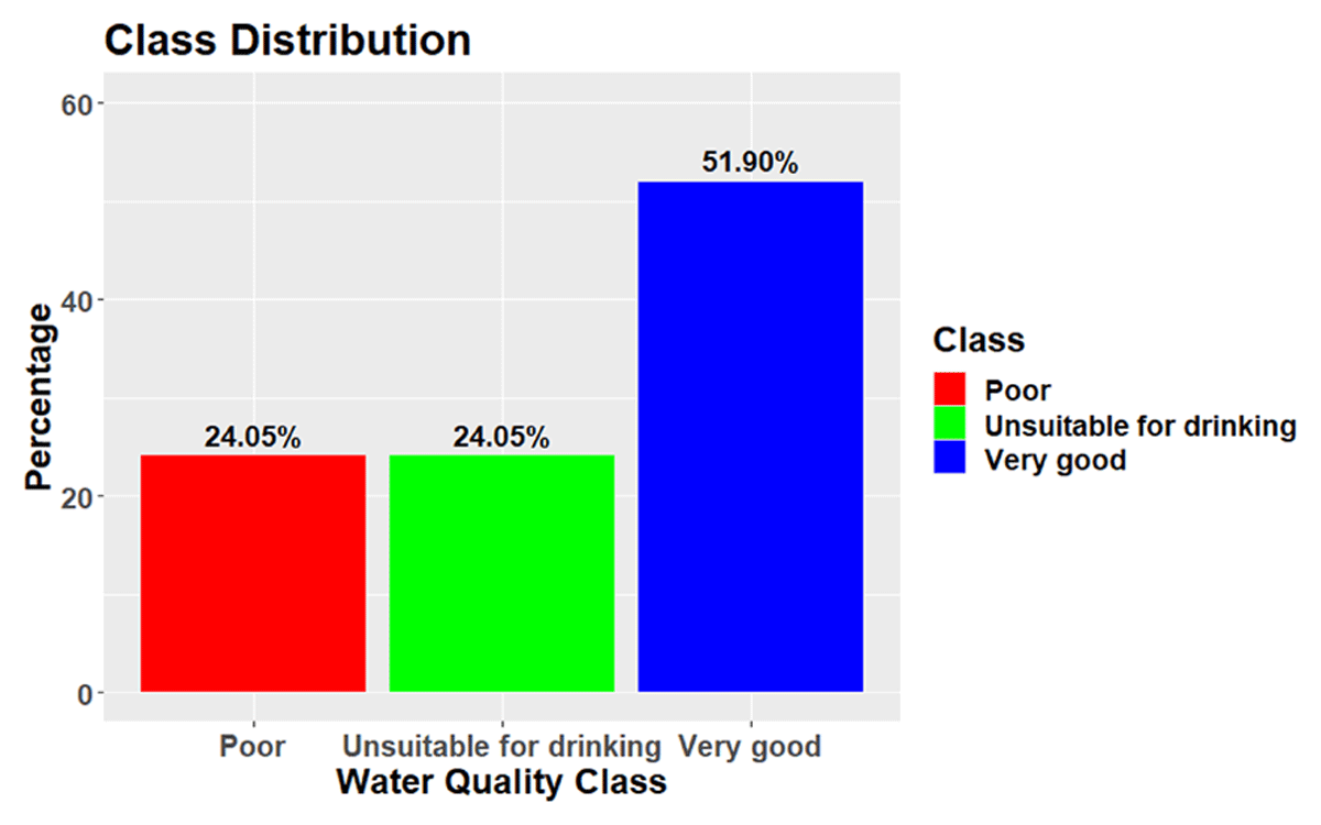
Figure 5
Visualizing the distribution of water quality classes.
Table 2
Descriptive statistics of water quality index deviation from the WHO value (Ilaboya et al., 2014; Khwaja and Aslam, 2018).
| S.NO | PARAMETERS AND HEAVY METALS | UNIT | WHO VALUE | ASSIGNED WEIGHTS | RELATIVE WEIGHTS | MEAN | SD | RANGE |
|---|---|---|---|---|---|---|---|---|
| 1 | Cd | mg/L | 0.05 | 4 | 0.12 | 0.04 | 0.01 | (0.01–0.07) |
| 2 | Cr | mg/L | 0.03 | 4 | 0.12 | 0.05 | 0.04 | (0–0.18) |
| 3 | Pb | mg/L | 0.01 | 4 | 0.12 | 0.19 | 0.29 | (0.01–0.91) |
| 4 | Ni | mg/L | 0.07 | 3 | 0.09 | 0.05 | 0.02 | (0–0.17) |
| 5 | Fe | mg/L | 0.3 | 3 | 0.09 | 0.05 | 0.02 | (0.02–0.13) |
| 6 | As | mg/L | 0.01 | 5 | 0.15 | 0 | 0 | (0–0) |
| 7 | Ph | Number | 6.5–8.5 | 4 | 0.12 | 7.74 | 0.25 | (7.3–8.6) |
| 8 | Ec | µS/Cm | 400 | 2 | 0.06 | 107.14 | 74.1 | (20–309) |
| 9 | TDS | mg/L | 500 | 5 | 0.15 | 53.98 | 39.7 | (9.5–193) |
Employing the Boruta algorithm, all parameters of the water, with the exception of arsenic heavy metal, were identified as more important and played a significant role in this study for the specific region of Khyber Pakhtunkhwa, Pakistan. Table 3 summarizes the key findings of the confirmed and rejected parameters and heavy metals with different descriptive statistics: ‘Mean-Imp’, ‘Range’, ‘Norm-Hits’, and ‘Decision’. Furthermore, we used different metrics for assessing the applied machine learning algorithms. Moreover, to ensure robust performance in this analysis, the dataset was divided into two parts, with 70% allocated to the training set and the rest to the testing or validation set. Subsequently, five supervised machine learning models were employed, including the DT model, the KNN method, neural network or the MLP algorithm, SVM, and the RF model to predict and classify the water quality class with multiple parameters and heavy metals. The overall model performance is checked by the final metric accuracy of the model, extracted from confusion metrics for each model. The DT model achieved an accuracy of 96% and 83% based on the training and testing sets, respectively. The KNN method achieved an accuracy of 75% with both the training and testing sets. The MLP achieved an accuracy of 96% and 83% based on the training and testing sets, respectively. SVM achieved an accuracy of 96% based on the training set and 88% with the testing set. Similarly, in our fifth effort, we employed the RF model, and the relative importance of each parameter or heavy metals was calculated, as shown in Figure 6. The RF model outperformed the previous models except for the SVM based on the testing set. The second comparable model is the SVM model according to the validation set. The RF model achieved 100% and 88% accuracy based on the training and testing sets, respectively, as shown in Figure 7. Furthermore, the summarization of various metrics like precision, recall, and F1-score are included in Table 4, providing insights through multiple comparison metrics for each model.
Table 3
Boruta algorithms based relative importance of water quality parameters and heavy metals.
| VARIABLE | MEAN-IMP | RANGE | NORM-HITS | DECISION |
|---|---|---|---|---|
| Cd | 12.89 | (11.51–13.84) | 1.00 | Confirmed |
| Cr | 15.79 | (13.77–17.46) | 1.00 | Confirmed |
| Pb | 24.74 | (22.14–27.06) | 1.00 | Confirmed |
| Ni | 10.13 | (8.96–11.65) | 1.00 | Confirmed |
| Fe | 11.03 | (9.51–12.05) | 1.00 | Confirmed |
| As | 1.02 | (–0.77–2.48) | 0.00 | Rejected |
| Ph | 3.59 | (1.53–4.99) | 0.76 | Confirmed |
| Ec | 13.27 | (12.01–14.92) | 1.00 | Confirmed |
| TDS | 15.14 | (13.34–16.51) | 1.00 | Confirmed |
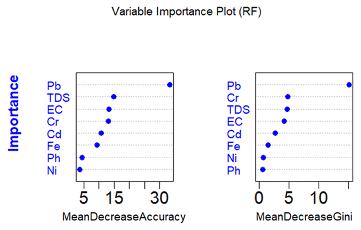
Figure 6
Ranking important parameters provides insights from the random forest model.
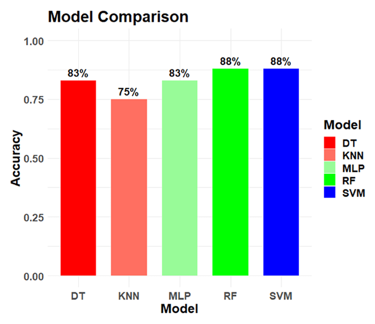
Figure 7
Evaluating accuracy metrics across various supervised machine learning models.
4. Conclusion
Water is essential for survival, so ensuring its quality is critical for our well-being. Traditional lab analyses, alternatively, may require more time and resources. Under these scenarios, establishing practical and effective ways to monitor water quality for this research study, such as using the WQI, becomes essential. The present study was conducted for the water quality evaluation in the three districts of Khyber Pakhtunkhwa, Pakistan, and employed supervised machine learning algorithms to predict and validate the WQI based on the various categories. This shows that most samples fall into the ‘Very good (51.9%)’ category, with 24.5% falling into the ‘Poor’ category and 24.5% falling into ‘Unsuitable for drinking water’ category. Based on the present study, we can conclude that half of the water in this area is fit for drinking, but we still need to be aware of the water quality management for the other parts of the remaining percentage. In a set of supervised machine learning models, all models perform well, but the RF outperforms in predicting the WQC based on both the training and validation sets, and the second comparable model is the SVM model. Based on the findings, we should consider integrating data from multiple locations in Khyber Pakhtunkhwa, Pakistan, to improve the capabilities of machine learning models for future studies. These methods can provide a fundamental understanding of the heavy metal parameters that affect water quality class. To ensure the long-term development of water quality in these locations, monitoring and protection actions must be prioritized, as well as actions to prevent further deterioration. The current study recommends that the government use appropriate measures, such as developed water monitoring systems and innovative technology, to address water quality issues in the influential areas of Pakistan.
Data Accessibility Statement
The data and codes used for the preparation of the manuscript are available with the corresponding author and can be provided upon request.
Ethics and Consent
All procedures followed were in accordance with the ethical standards with the Helsinki Declaration of 1975, as revised in 2000.
All authors voluntarily agreed to participate in this research study.
All authors are agreed to for publication. There is no legal constraint in publishing the data used in the manuscript.
Competing Interests
The authors have no competing interests to declare.
Author Contributions
All authors contributed equally.