
1 Introduction
Many physical systems are governed by principles that can be expressed in terms of differential equations. In the case of a system with a multi-dimensional state vector x, the evolution of x is described by a set of differential equations, each taking the form:
x is a component of x, which is a function of time t. The differential forcing F(x(t)) is a deterministic function of x. F(x(t)) describes internal dynamics arising from interactions of x with other components of x under the influence of some external forcings. Examples of systems governed by equations in form of Eq.(1) include a climate model describing the atmosphere and the ocean, and a many-particle system describing the movements of Brownian particles suspended in a fluid. A common feature observed from these physical systems is the lack of serial correlations, where a solution at one time point is uncorrelated to the solution at another more distant time point. A solution that lacks serial correlation is commonly regarded as random. We identify this randomness as the subject of this study. Under this definition of randomness, movements of a Brownian particle are random; weather patterns are random. Random features are also found in many other occasions. A prominent example in atmospheric sciences concerns time averages of meteorological variables. These averages display variability similar to that of the sample mean of a random variable, leading to the concept known as “climate noise” (Leith, 1973; Madden, 1976, 1981; Feldstein & Robinson, 1994; Feldstein, 2000). Despite evident random behaviors found for classical physical systems, a theory of randomness is still missing.
Instead, heuristic arguments are used to provide some explanations. Such arguments often associate randomness with uncertainties. Two types of uncertainties are considered in this context. The first one arises from our inability to precisely track the evolution of each individual degree of freedom in a system that has an exceedingly large number of degrees of freedom. Brownian motion serves as a typical example, as it is challenging to formulate and to solve the complete set of equations that describe all interactions between fluid molecules and Brownian particles. The standard approach, commonly used to deal with noise and fluctuations in physical systems (MacDonald, 1962), is to replace the original deterministic equations by ones that include stochastic forcing. In case of Brownian motion, the original equations are replaced by Langevin-type equations.
Inspired by the statistical approach used for handling Brownian motion, Hasselmann proposed to describe climate variability using stochastic climate models (Hasselmann, 1976). These models are formulated for the slow components of x. In line with the statistical treatment of slow Brownian particles embedded in fast fluid molecules, a stochastic climate model for a slow component x is written as
represents the slow dynamics of x and the averaged effect of the fast components of x on x, with being an average over a time period longer than the timescale of the fast components but shorter than the timescale of x. ζ is a stochastic forcing used to describe the fluctuating effect arising from the fast components.
Statistical approaches are efficient in constructing different variance-generation mechanisms. In case of Hasselmann’s stochastic climate model, a solution obtained by integrating Eq. (2) over time contains an integral of ζ over time, which is a random walk. The variance of a random walk increases with increasing time. In order to obtain a stationarily varying solution from Eq. (2), must incorporate negative feedbacks (Hasselmann, 1976). Thus, variations generated by a stochastic climate model result from the joint effect of random-walk and negative feedbacks. Statistical approaches can also be accurate in describing random behaviors, if the stochastic forcing is carefully constructed to possess specific properties. What statistical approaches do not explicitly address is the mechanism responsible for the randomness in solutions of the considered system.
The other type of uncertainty arises from our inability to specify the exact initial conditions from which the considered physical system starts to evolve with time. This problem, first described by Lorenz (1963) and well-known to the numerical weather forecast community, is one of the key aspects studied by the dynamical systems theory. There, the sensitivity to initial conditions is attributed to the chaos arising from non-linear dynamics in a dynamical system. However, dynamical systems theory does not explicitly deal with randomness. It is unclear whether and to what extent chaotic solutions are random.
Quite the contrary, both the statistical approaches for handling high-dimensional systems and the investigation addressing the sensitivity to initial conditions implicitly assume that a physical system is fundamentally deterministic. The situation is understandable, since the uncertainties, which represent randomness, do not originate from the deterministic dynamics. Instead, they result solely from external factors related to our inability in tracking the exact solution or in specifying precise initial conditions. This assumption about determinism is in obvious conflict with the randomness which we experience from physical systems.
One step towards resolving this conflict is made by the finding that the determinism, as dictated by Eq. (1), breaks down under certain circumstances (von Storch, 2022). Given Eq. (1), the spectra of x and F, Γx(ω) and ΓF(ω) where ω is frequency, are related to each other via
Eq. (3) seems to confirm the determinism that variations of x at any one frequency must be generated by the variations of F at the same frequency. This however cannot be true for a solution whose spectrum Γx(ω) is continuous and approaches a finite and non-zero Γx(0) as ω → 0. Given a finite and non-zero Γx(0), Eq. (3) requires that ΓF(ω) must go to zero as ω → 0 so that ΓF(0) = 0. Thus, at frequency ω = 0, variations of x can not be generated by variations of F at this frequency.
Before elaborating the meaning of the just mentioned low-frequency shape of Γx(ω), we point out that the determinism described by Eq. (3), which holds for all frequencies except zero frequency, is the norm that can become more prominent in case when F contains a time-varying external forcing. The present paper does not question and is not concerned with this determinism. To concentrate on internal dynamics, in which the origin of randomness presumably lies, we will focus on physical systems that are not influenced by any time-varying external forcing. We cannot rule out the presence of constant external forcings, as variations in a physical system, no matter random or deterministic, necessitate external power support.
Come back to the low-frequency shape of Γx(ω). That Γx(ω) is continuous and has finite and non-zero spectral value as ω → 0 describes nothing other than the manifestation of randomness in the solution of x. When defined as a Fourier cosine transform of auto-covariance function, the spectrum of a solution Γx(ω) only exists when the auto-covariance function is absolutely summable. Upon existence, Γx(ω) must be continuous, since a cosine function is continuous and since a Fourier cosine transform is a sum of weighted cosine functions. The condition of absolute summability implies that the auto-covariance function must decay to zero with increasing time lag. It is precisely this decay of auto-covariance function that diminishes serial correlation and makes a solution to appear random. It is also this decay of auto-covariance function that prohibits the solution of x to be purely periodic. Auto-covariance function of a purely periodic solution, whose spectrum consists of distinct spectral lines (Priestley, 1981), does not decay and retain its magnitude as time lag increases. It is still this decay of auto-covariance function, that allows Γx(0), the value of Γx(ω) at ω = 0, to be finite and non-zero. To see this, note that being a Fourier cosine transform of an auto-covariance function and since the value of a cosine function at the origin is one, Γx(0) is identical to the sum over the auto-covariance function at all time lags. Given that an auto-covariance function has a positive maximum at lag zero, the sum of an auto-covariance function that decays with increasing time lag can lead to a Γx(0) that is not zero and finite. The same argument does not apply to ΓF(0), since auto-covariance function of F consists of differences of auto-covariance function of x because of Eq. (1) (von Storch, 2022).
The finite and non-zero low-frequency shape of Γx(ω) can be inferred from spectra of variables that are apparently random. Figure 1 shows a collection of such spectra. To this end we note that while the deterministic influence of external forcing can be easily controlled in a numerical experiment, achieving the same for the real climate is challenging. The real climate is subjected to an external forcing, that has a non-zero mean and varies with time. The real climate can hence reveal not only random behaviors resulting from internal dynamics (via e.g. instability and turbulence), but also deterministic behaviors resulting from external forcing. The latter includes for example long-term trends as responses to a slowly varying external forcing, and oscillations (e.g. annual cycle) as responses to a periodic external forcing. Thus, if we want to find from observations spectra that are continuous and have finite and non-zero values at the lowest frequencies, we need to consider those variables whose variations are mainly generated by internal dynamics, with the influence of external forcings being negligibly small relative to that of these internal dynamics.
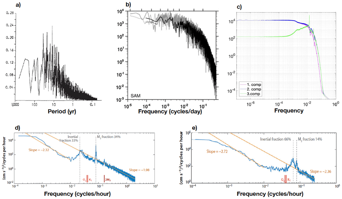
Figure 1
Spectra of a) a spherical harmonic coefficient simulated by an atmospheric model (James & James, 1989), b) zonally averaged SLP difference representing the Southern Annular Mode from the NCEP/NCAR reanalysis (solid black) and from models (gray) (Deser et al., 2012), c) the three components of the Lorenz’s 1963 model (von Storch, 2022), d) and e) current kinetic energy from instrumental records in the North Atlantic at 500 m and in the South Pacific at 1000 m (Ferrari & Wunsch, 2009). Using detrended time series (dashed black line in b) can be considered as a way to eliminate the influence from external forcings.
Figure 1a) shows a spectrum of a component x of a dry atmospheric model (James & James, 1989), generated by model’s internal dynamics without influence of any time-varying external forcing. Figure 1b) shows spectra of sea level pressure derived from an atmospheric reanalysis (Deser et al., 2012) (black lines). Figure 1d) and e) show spectra of current kinetic energy derived from instrumental records (Ferrari & Wunsch, 2009). We assume that sea level pressure and ocean current are variables whose variations arise mainly from internal dynamics. All these spectra reveal finite and non-zero values at the lowest resolved frequencies. Finally, Figure 1c) shows the spectra derived from the Lorenz model (Lorenz, 1963), a model that does not contain any time-varying external forcing. In contrast to the other spectra depicted in Figure 1, which are merely indicative owing to the limited duration of available observations and model solutions, the finite and non-zero low-frequency shape of Γx(ω) can now be demonstrated asymptotically by considering longer and longer Lorenz solutions (von Storch, 2022). We conclude that for a solution of a system governed by a set of equations in form of Eq. (1), the apparent randomness is manifested in the solution’s spectrum that is continuous and has a finite and non-zero Γx(0). This spectral feature enforces the breakdown of determinism at zero frequency, including the associated asymptotic behavior towards the breakdown at near-zero frequencies. The breakdown suggests that Γx(0) has nothing to do with F, which is puzzling at first glance.
On further reflection, we notice that the randomness in x and the wholly deterministic nature of F do not pertain to the same thing. Randomness in x is only evident when a solution of x at time t is set in relation to the solution of x at a distant time t+T with T ≠ 0. A Brownian particle appears to move randomly because its velocity at time t seems to be independent of its velocity at time t+T, where T is a time interval larger than the reaction time of the human eye. F on the other hand tells us about the evolution tendency. Given F of the velocity of a Brownian particle at time t (which is a function of the whole state vector x describing the positions and velocities of all involved particles and molecules at time t), the time rate of change of the velocity of the considered particle is know exactly. Nothing is random. Thus, if we want to understand the mechanism behind the randomness, we should shift to examining the integral forcing GT, a definite integral of F(x(t)) over a time span of length T that drives the evolution from x(t) to x(t+T). Studying GT contrasts with the standard approaches that emphasize solely the differential forcing F.
This paper explores the properties of GT(t). Following some preliminaries provided in Section 2, we show in Section 3 that GT consists of a fluctuating and a dissipating components, in accordance with the fluctuation-dissipation theorem of Callen and Welton (1951). This theorem was introduced to the realm of climate research by Leith (1975) who showed how the theorem can be used to estimate climate responses to a changing external forcing, no matter which component x of x is considered. We show that there exists a threshold such that for T larger than this threshold, GT emerges as a unified forcing. Section 4 describes the impacts of these properties of GT on the solution of x. Section 5 and 6 discuss two aspects that are essential for the dissipation represented by GT. Conclusions are provided in Section 7.
2 Preliminaries
2.1 Continuous solutions
Consider a physical system, whose evolution is governed by a set of equations in form of Eq. (1). Suppose that this set of equations has a solution and the solution at time t is x(t). This solution is a function of continuous time, and referred to as a continuous solution. For component x of x, its differential forcing F(t) = F(x(t)) is also a function of continuous time. Its integral forcing GT(t) at time t is defined as the definite integral
where represents the non-negative part of the real axis. Being an integral of F which is a function of the full state vector x, GT(t) can only be obtained after the whole system has been integrated over the interval [t,t+T). For T = 0, GT(t) = 0. For T < 0, GT(t) is not defined.
Following Section 1 and throughout this paper, a solution of x, x(t), is deemed random when x(t) is independent of x(t+T) for any time t and for all T larger than a threshold. The evolution from x(t) to x(t+T) is determined by GT(t) defined in Eq. (4). To understand what makes x(t) independent of x(t+T), we explore properties of GT(t) for different values of T. We do so systematically by grouping the states at separated time points along a solution according to the time span that separates the time points. When setting the initial time of the solution at zero, such a group forms a series , where T denotes the length of the time span, x(iT) denotes the solution of x at time t = iT, and is the set of non-negative integers. The integral forcing, which is responsible for the evolution from one member to the next in the series , constitutes the series , where GT(iT) is obtained by setting t = iT in Eq. (4). We have for any
Both and are discrete series, with their members being defined at discrete times t = iT with .
2.2 Discrete solutions
For a real physical system, the set of governing equations in form of Eq. (1) often does not have analytical solutions, and must be solved numerically by discretizing the time axis using a time increment Δt. The resulting solutions are referred to as discrete solutions. A discretized version of Eq. (1) takes the form
Integer j counts the j-th time step at t = jΔt. xj is a component of the solution xj at the j-th time step, and Fj = F(xj). Following Eq. (4), the integral forcing of x at the k-th time step, Gτ,k, is defined as the integral over Fj at τ time steps starting from the k-th time step:
is the set of positive integers. Similar to GT(t), Gτ,k can only be obtained by integrating the whole system forward in time. Different from GT, which is a function of continuous solution, Gτ is a function of discrete solution. Gτ is not defined for τ ≤ 0.
Again, to understand the behaviors of a solution at separated time steps, we explore the properties of Gτ,k for different values of τ. To do so, we group the states at separated time steps along a solution according to the number of time steps covering the separation. Setting again the initial time of a discrete solution at the origin, such a group forms a series , where τ denotes the number of time steps covering the separation, and xiτ is the solution at the (i × τ)-th time step. The integral forcing, which is responsible for the evolution from one member to the next in the series , constitutes the series , where Gτ,iτ is obtained by setting k = iτ in Eq. (7). We have for any value of ,
We note that as a consequence of discretization, Gτ,iτ is not defined for τ = 0 and equals FiΔt for τ = 1. Provided that Δt is reasonably small, we assume that the properties of Gτ can be considered as the properties of GT. We describe these properties in term of Gτ, since they can only be verified when knowing the solution of x, and since for systems of our interests, only discrete solutions are available.
3 Properties of integral forcing
Important for the consideration below is the condition of a physical system referred to as equilibrium. This condition can be achieved under the influence of constant external forcings. For a multi-dimensional system, an equilibrium is generally not described by a solution that is independent of time, but by a solution that varies stationarily with time. If the external influences were kept constant forever, the solution would continue to vary stationarily into infinite times. In case of a climate model, an equilibrium of the model can be reached by integrating the model under constant external forcing conditions for some time (to allow the model to spin up).
Consider a multi-dimensional system in equilibrium. For every component x of the system’s state vector x, and for any , the properties of the integral forcing of x, , are described by the following three postulates.
I. Gτ,iτ consists of, apart from a constant , a dissipating component and a fluctuating component fτ,iτ, and can be written as
and are the intercept and the slope of the line obtained by regressing Gτ,iτ against xiτ using n pairs of (xiτ,Gτ,iτ) along a solution, where n is finite. fτ,iτ, the residual not described by the regression line, is determined such that Gτ,iτ in Eq. (9) is identical to Gτ,iτ in Eq. (8) calculated from Eq. (7).
II. The expression given in Eq. (9) is unique in the sense that it can be replaced by
where
Moreover, the dissipating and fluctuating components are related to each other via
where is the variance of the series and is the variance of the series . On the plane spanned by dτ and or the plane spanned by dτ and , Eq. (12) is a curve that has its maximum at the center where dτ = –1 and is mirror symmetric about dτ = –1. Such a curve is referred to as a fluctuating-dissipating curve, or for short a fd-curve.
III. There exists a threshold τ0 such that Gτ,iτ with τ > τ0 emerges as a unified forcing consisting of a dissipating component characterized by dτ = –1, and a fluctuating component fτ,iτ that behaves like a white noise.
Postulate I, which is the basis of all postulates, adopts the idea behind the fluctuation – dissipation theorem (Callen & Welton, 1951) that for a system in equilibrium, anything that generates fluctuations must also damp the fluctuations. In case of the Brownian motion, the collisions with fluid molecules make a Brownian particle to fluctuate. At the same time, the collisions introduce a drag that damps the movement of the particle. Postulate I says that for a system in equilibrium, Gτ always contains a dissipation, independent of the value of τ and no matter which one of the components of x is considered. Whether this is true is a priori not clear.
To verify these postulates, we need many long series {xiτ|i = 1,2,…} and {Gτ,iτ|i=1,2,…}, for many different values of of τ. Despite the advance of computer technology, numerically deriving all these long series is still challenging for a high-dimensional system, such as a climate model or a Brownian system. We hence verify these postulates in terms of the Lorenz model (Lorenz, 1963). This model is multi-dimensional and possesses an equilibrium described by stationarily varying and seemingly random solutions.
3.1 Verification of Postulate I
Formally, Gτ,iτ can always be described by the expression given in Eq. (9) using a properly chosen fτ,iτ. Since no conditions have been imposed on fτ,iτ, apart from its existence, Postulate I is verified by showing that is negative for all components of x and for all τ ≥ 1. Figure 2 shows for the three Lorenz components (magenta, blue and green) and for five values of τ that the regression line is indeed always tilted with a negative slope. The exact values of are truncated to two digits after the dot and listed in the bottom left corner of each scatter diagram. Negative slopes are also found for all other considered values of τ, as shown by Figure 5.
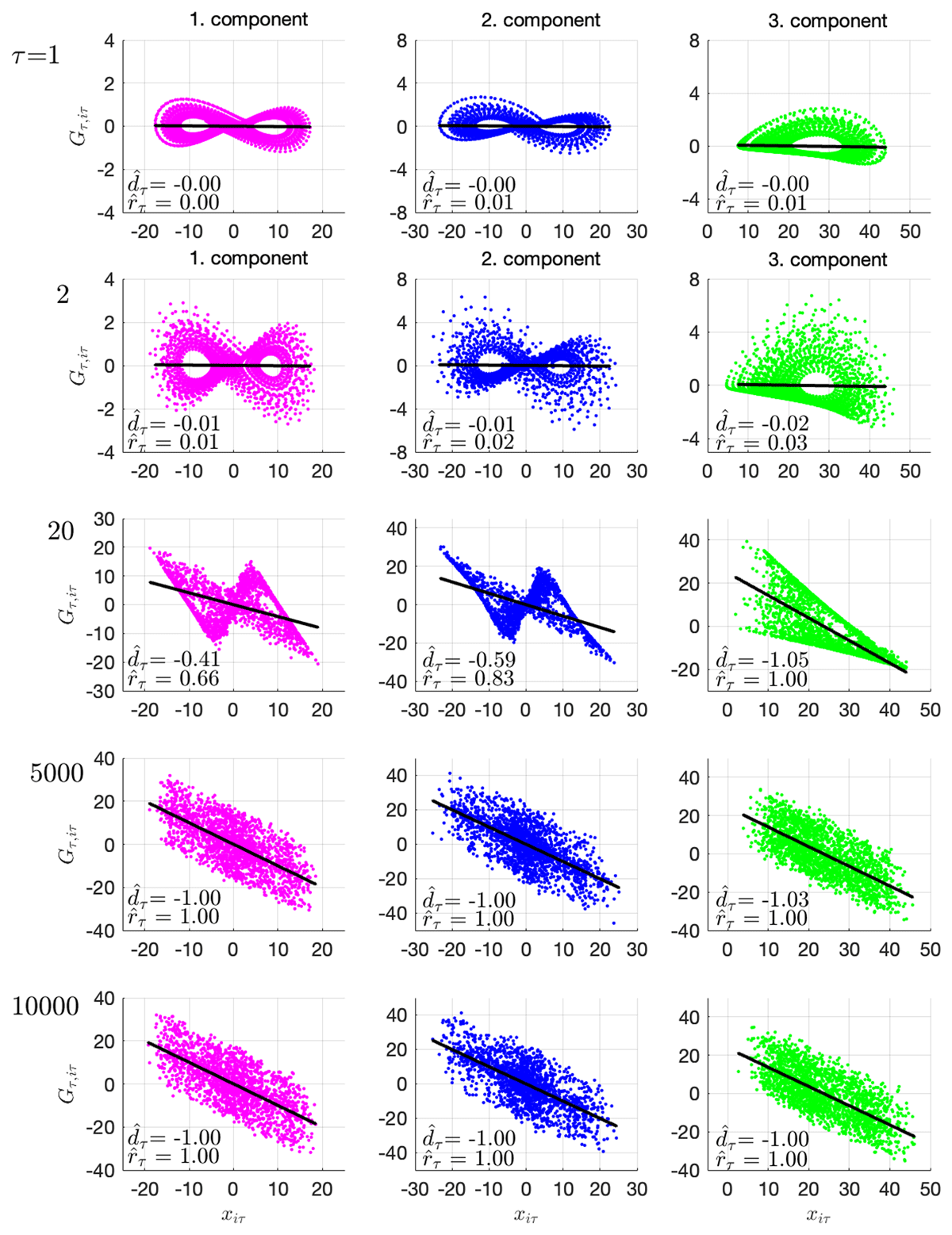
Figure 2
Scatter diagrams of Gτ,iτ against xiτ (dots) and the respective regression lines (black lines) for five values of τ (listed on the far left) and for the three Lorenz components (magenta, blue, green), as derived from n = 106 pairs of . , and are calculated following Eq. (A1) – Eq. (A4) in Appendix A. Numbers listed in each scatter diagram are values of and , where is the variance of and is the variance of . Points (xiτ,Gτ,iτ) are collected along a stationary Lorenz solution. A stationary Lorenz solution is obtained by first integrating the Lorenz model from an arbitrary initial state for a sufficiently long time. The integration is done using a Runge Kutta scheme with a time step of 0.01.
3.2 Verification of Postulate II
Postulate II is verified in terms of Figures 3 and 4. Figure 3 shows for all three Lorenz components and for two different values of τ that and converge with increasing n, the number of data points used for calculating the regression line. The convergences suggest that both and exist. Gτ,iτ can hence be uniquely expressed in terms of Eq. (10). The notions and are still used, since everything we show are derived from a finite number of data points along a solution.
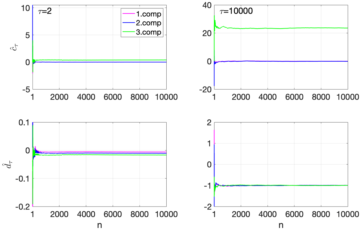
Figure 3
(top) and (bottom) for τ = 2 (left) and τ = 10000 (right) and for the three Lorenz components (magenta, blue and green) as functions of n, the number of pairs (xiτ,Gτ,iτ) used for their calculations. The calculation is carried out using an increment in n that equals one for 1 ≤ n ≤ 500 and equals 20 for 500 ≤ n ≤ 10000.
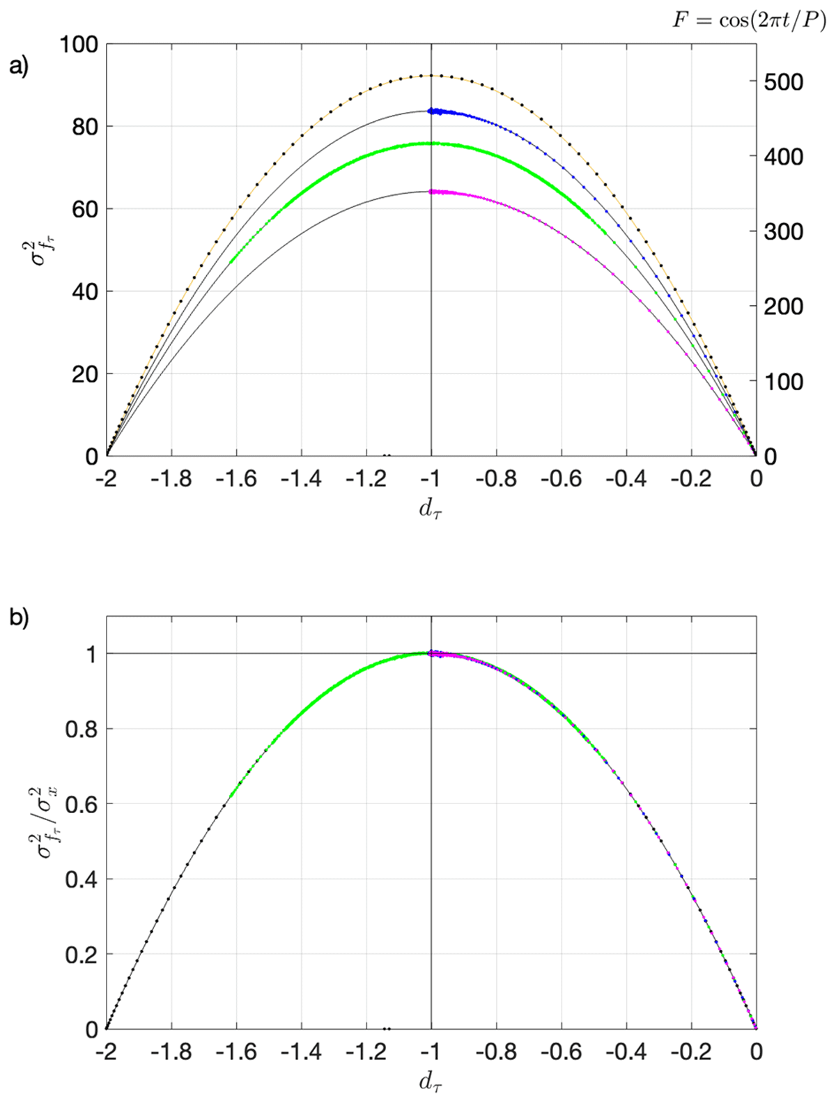
Figure 4
(top) and (bottom), with being set to the variance of each of the three Lorenz components (black lines) and to the variance of the solution of dx/dt = cos(2πt/P) with period P = 200 (orange line). The latter equals P2/(8π2) = 506.61. Colored dots are points (top) and points (bottom) with τ = 1,…,1000, each obtained using n = 106 pairs of (xiτ, Gτ,i) along a stationary Lorenz solution, with the colors (magenta, blue, and green) indicating the Lorenz components. Black dots are points with T = 1,2,…,P, obtained from (x(iT),GT(iT)) with i = 1,…, 5P. Both x(iT) and GT(iT) are calculated using the analytical expressions obtained from the cosine model. dT and are calculated using the regression defined in the same way as for the discrete solution.
Figure 4 shows the fd-curves complemented by the variances of the three Lorenz components (black lines). For all three Lorenz components, the points (magenta, blue, and green dots) are located right on the fd-curve (top); and the points with normalized variance, , are located right on the fd-curves (bottom). Thus, the relation between and can be readily described by Eq. (12) for a large but finite n. Appendix B shows further how Eq. (12) emerges in the limit n → ∞.
Regarding the points or , there is a difference between the three Lorenz components. As τ increases, the points of the first two Lorenz components (magenta and blue dots) move from the right end to the center of the fd-curve, and eventually stay and remain to stay at the center of the curve. strengthens monotonically from zero to –1 with increasing τ, and equals –1 for τ larger than a threshold. For the third Lorenz component, the points (green dots) move with increasing τ from the right end of the curve toward the left, pass the center of the curve, and reach the most left position at . As τ further increases, they move backward toward the right, pass the center of the curve, and reach the most right position at . Thereafter, they continue to move back and forth around the center of the fd-curve, with the far left and the far right position reached becoming increasingly close to the center the fd-curve. As a result, strengthens from zero to –1 in a non-monotonic manner.
3.3 Verification of Postulate III
Postulate III is verified by Figures 5 and 6. The two figures show that for all three Lorenz components, there exists a threshold τ0 such that for τ > τ0, Gτ,iτ represents a unified forcing. The phrase “unified” refers to the same type of Gτ,iτ, no matter which component of x is considered, and independent of values of τ provided τ > τ0. This unified forcing contains a dissipating component that is characterized by dτ = –1 and a fluctuating component whose auto-correlation function resembles that of a white noise. The threshold τ0, beyond which the unified forcing is found, depends on the component x considered. It is smaller for the first two Lorenz components (magenta and blue) than for the third Lorenz component (green).
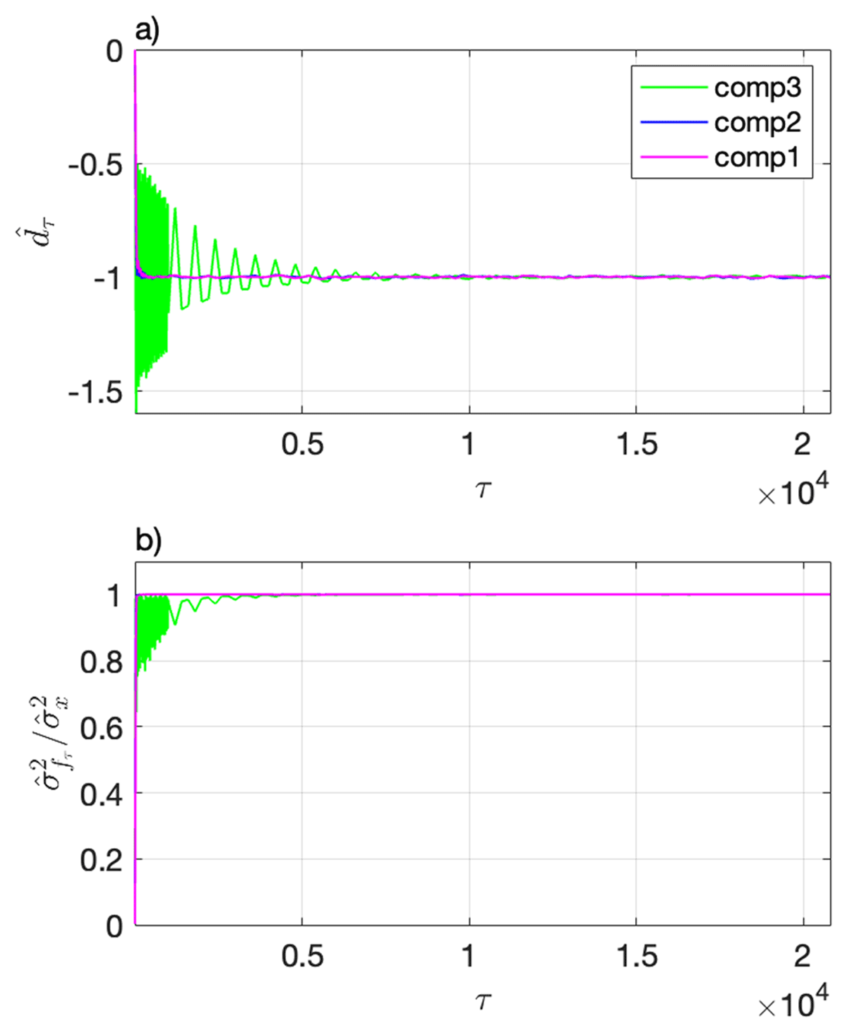
Figure 5
and as functions of τ, derived using n = 105 pairs of (xiτ,Gτ,iτ) along a stationary Lorenz solution. and obtained from the first two Lorenz components (magenta, blue), which overlay each other, converge with increasing τ faster than those obtained from the third component (green). The calculation is done using an increment in τ that equals 10 for 1 ≤ τ ≤ 1001 and equals 200 for τ >1001.
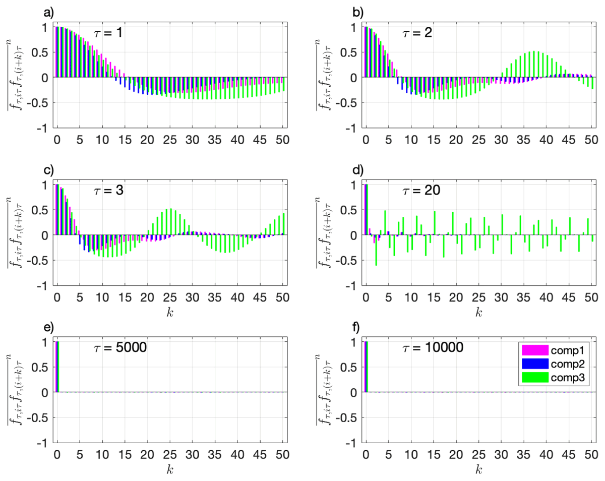
Figure 6
Auto-correlation function of fluctuating component , defined as , for six values of τ, obtained for the three Lorenz components (magenta, blue, green) using n = 106 data points along a stationary Lorenz solution. is a function of k. The smallest non-zero time lag resolved by is obtained for k = 1, corresponding to a time lag of τ time steps.
By definition, Gτ,k is the sum over Fj at τ time steps obtained when integrating the whole system from time step k to time step k+τ –1. Before Gτ,k with dτ = –1 is produced, the forward integration first produces G1,k = FkΔt, then G2,k = FkΔt+Fk+1Δt, and so forth, and eventually . Thus, we should see a general strengthening of the dissipating component, characterized by an overall increase from |d1|, to |d2|, and so forth, before the maximum characterized by |dτ| = 1 is reached. A sign of this can already be seen from Figure 2, which shows a general strengthening of dτ with increasing value of τ (from top to bottom row in Figure 2).
For τ < τ0, the way how the dissipating component of Gτ,iτ strengthen with increasing τ is different for different Lorenz component. While the strengthening is monotonic for the first two Lorenz components, it is non-monotonic for the third Lorenz component. The former is characterized by the uni-dimensional movement of the -point along the fd-curve with increasing τ described before, which results in the magenta and blue lines in Figure 5. The latter is characterized by the back and forth swing of the -point along the fd-curve, which results in the green lines in Figure 5.
4 Impacts of integral forcing Gτ
The dissipation, that is associated with Gτ and characterized by dτ, is the same between any two adjacent members in the series . As such, it systematically weakens the link between xiτ and xiτ+τ, resulting in an auto-correlation function of x at lag τ, ρτ, whose magnitude is smaller than one. This relation between dτ and ρτ (see Appendix C for its derivation) is described by
Although presented as an equality, ρτ should be regarded as the effect resulting from dτ, since xiτ+τ that has a weaker link to xiτ is generated by Gτ,iτ that diminishes xiτ by the amount quantified by |dτ|.
For Gτ with τ > τ0, Gτ,iτ = cτ+ dτ xiτ +fτ,iτ is replaced by
with fτ,iτ being a white-noise-like forcing. With Eq. (14), Eq. (8) reduces to
xiτ+τ becomes independent of xiτ, a behavior deemed as random in Section 1. We hence conclude that it is the integral forcing Gτ of x with τ > τ0, that makes the solution of x to become random. Given Eq. (15), the variance of the series , which equals also the variance of the series , becomes identical to the variance of . Consequently, the ratio is identical to one, as shown in Figure 5b).
Furthermore, for any two adjacent members in the series , it is impossible to determining the past member xiτ from the future member xiτ+τ, despite of Eq. (8). This is because as Gτ,iτ with τ > τ0 emerges through forward integration, the dissipating component of Gτ,iτ cancels with the past state xiτ little by little and eventually completely, at the time when xiτ+τ is generated by the fluctuating component fτ,iτ of Gτ,iτ at time step iτ+τ. Consequently, xiτ is independent of fτ,iτ. This independence leads to a parallelogram-like shape of the scatter obtained when regressing Gτ,iτ against xiτ (two bottom rows of Figure 2). The evolution from xiτ to xiτ+τ is not only random but also irreversible.
The relation between two adjacent members in the series with τ > τ0 is in striking contrast with the relation between x(t) and x(t+δt) with an infinitesimal δt for a continuous solution, or the relation between xk and xk+1 for a discrete solution. Given F(x(t)), Eq. (1) is also valid when time is reversed. Given Fk, Eq. (6) can be integrated for a given past state xk forward in time to predict the future state xk+1, or integrated for a given future state xk+1 backward in time to predict the state member xk. The evolution from x(t) to x(t+δt) with an infinitesimal δt is reversible, so does the evolution of from xk to xk+1. The key to the reversibility is the differential forcing F(x(t)), or Fk, which represents a forcing rate at a time instant. This stands in stark contrast to Gτ,k, which is a forcing over a time span of non-zero length.
5 Significance of passing of time
A further aspect that makes Gτ different from F concerns the dissipation represented by Gτ, which should not be confused with the damping included in F. We refer the latter as “damping” to distinguish it from the dissipation in Gτ. In the Lorenz model, F contains a linear damping ax with a = –10, –1, and –8/3 for the three components respectively. The damping in F differs from the dissipation in Gτ. Being a differential forcing, the strength of the damping (i.e. a in the Lorenz model) represents a damping rate, and has the unit of 1/[t], with [t] being the unit of time. Different from that, the dissipation in Gτ, which is characterized by dτ, represents a portion of dissipation and is dimensionless. More importantly, the damping in Fj is not associated with any specific timescale, consistent with the fact that it represents a rate, whereas dτ is associated with one and only one timescale of length τΔt. dτ represents the dissipation experienced by an evolution of x from xk to xk+τ over τ time steps.
We further explore the difference between the damping in F and the dissipation in Gτ using the Lorenz model. In this paper, the Lorenz model is solved using Δt = 0.01. With this value of Δt, the damping within one time step, aΔt, equals –0.1, –0.01, and –0.027 for the three Lorenz components, respectively. Here, we have disregarded the impact of the numerical scheme used for solving the discretized equations, which can affect the damping amount by a few percent. The values of aΔt can be compared with the dissipation experienced by x as x evolves from xi to xi+1 over a time span of length Δt, which is quantified by d1 and listed in the first row of Figure 2. We find that the values of aΔt are much larger than the values of d1.
We further explore the difference between the damping in F and the dissipation in Gτ by considering the limit Δt → 0. In this limit, Eq. (6) converges to Eq. (1), and d1 converges to dT with T = 0 defined for a continuous solution. Since for T = 0, GT(t) = G0(t) = 0 for all dT with T = 0 must also be zero. However, the fact that d1 → 0 in the limit Δt → 0 does not make d1 so different from the damping within one time step, aΔt, since we have also aΔt → 0 in the limit Δt → 0. The difference between the damping in F and the dissipation in Gτ becomes only apparent when considering the rate of dissipation and the rate of damping. Figure 7 shows that aΔt is proportional to –Δt, whereas d1 is proportional to –Δt2. Thus, the dissipation rate vanishes,
whereas the damping rate
is generally not zero. Eq. (16) and Eq. (17) suggest that the damping in F and the dissipation in Gτ are two different things. The dissipation in Gτ cannot be included in F as a forcing rate, since this rate vanishes exactly.
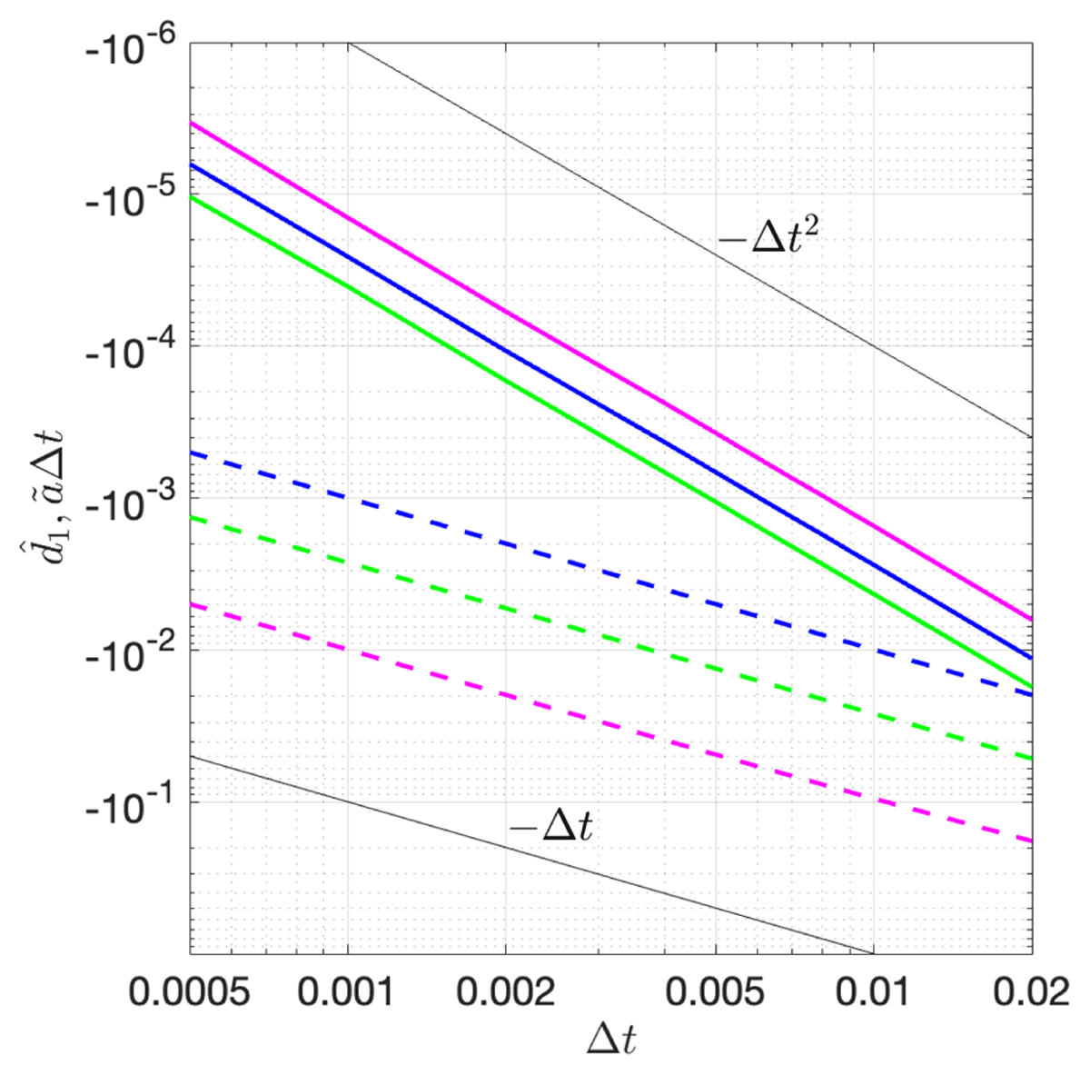
Figure 7
Dissipation associated with integral forcing G1 (i.e. Gτ with τ = 1, solid lines) and damping amount due to differential forcing F (dashed lines) as functions of time increment Δt, for the three Lorenz components (magenta, blue, and green). The dissipation associated with G1 is quantified by . For a given value of Δt, is the regression slope obtained by regressing G1,i against xi using (xi, G1,i) with i = 1,…,106 along a Lorenz solution computed with this Δt. The damping amount due to F is quantified by ãΔt, where ã is the proportionality factor of the linear damping in the discretized Lorenz model. The values of ã differ slightly from a = –10, –1, –8/3 given in the Lorenz model. The difference results from the numerical scheme used, which is the fourth order Runge-Kutta scheme in this study. The two black lines are proportional to –Δt and –Δt2, respectively.
Given the link of dτ to the specific timescale of length τΔt, we may interpret the dissipation in Gτ,k as something that results from interactions of xk with other components of x, that have taken place within a time span covering τ time steps starting from the k-th time step. The length of the time span is τΔt. For τ = 1 and when Δt goes to zero, the length of the time span, τΔt = Δt, goes to zero. No interaction of x with other components of x can complete within a time span of vanishing length. d1 approaches zero. On the other hand, increasing the value of τ for a given Δt increases the length of time span τΔt. The larger the value of τ, the more interactions between xk and other components of x can take place within the time span extending from the k-th to the (k+τ-1)-th time step, the stronger is the dissipation resulting from these interactions. The threshold τ0, beyond which Gτ equals the unified forcing, corresponds to the length of the time span that starts from the k-th time step and encompasses all interactions, and only these interactions, between xk and other components of x. Further extending the length of this time span (by increasing τ) allows more interactions to occur within the time span. However the additional interactions no longer involve xk at the k-th time step and hence no longer contribute to the dissipation of xk.
Accepting the idea of the fluctuation – dissipation theorem that for a system in equilibrium, anything that generates fluctuations must also damp the fluctuations, this “anything” is manifested in actions that take place in form of interactions of x with other components of x. Without the passing of time, these actions cannot be completed and the associated dissipation cannot take effect. The demand on the passing of time is in stark contrast to the damping in F, which is a forcing rate needed to balance the rate of external forcing, and exists without the passing of time.
6 Significance of multi-dimensionality
The interpretation of the timescale dependence of dτ suggests that multi-dimensionality is a necessarily condition for Gτ to possess a dissipation that allows Postulate III to be valid, and with that a solution that is random. Even though we are unable to prove this assertion rigorously, we provide below some supporting evidences. We do so by considering two one-dimensional systems as counterexamples, for which Postulate III is not valid, and consequently whose solutions cannot be random.
The first example is the one-dimensional system , where β is a constant. This system has the analytical solution x(t) = x0+βt. The differential forcing of x is β; the integral forcing of x is GT(t) = βT. For a given non-zero value of T, the regression slope dT obtained from regressing GT(t) against x(t) is zero, since GT(t) is independent of t and then independent of x(t), no matter whether β is positive or negative. With dT = 0, GT(t) does not contain a dissipating component. Postulate I is not valid. Without Postulate I, the other two postulates, especially Postulate III, are meaningless. The solution x(t) = x0+βt is always deterministic.
The second example is the one-dimensional cosine model, with period P. This model has the analytical solution . The differential forcing of x is cos(2πt/P); the integral forcing of x is . Figure 8 shows for six values of T and for t = iT and i = 1,…,n, how GT(t) are scattered against x(t). Also shown are the regression line GT(iT) = cT+dT xiT + fT,iT for each value of T. In all six cases, the regression lines are tilted with a slope dT < 0, albeit dT with a value of T that is close to a multiple of P (as in Figure 8a, f) is close to zero and has to be listed as –0.00 when keeping only two digits after the point. The negative slope is also found for T = P/4 (Figure 8d), for which the period of GT(iT) is four and the regression line goes through only four pairs of (xiT,GT(iT)). Thus, the integral forcing GT(iT) can also be decomposed into a dissipating and a fluctuating component for a periodic solution. Postulate I is valid for the cosine model. The idea that for a system in equilibrium, anything that generates fluctuations must also dampen those fluctuations, seems to apply universally to all types of stationarily varying solutions, regardless of whether they are periodic or non-periodic.
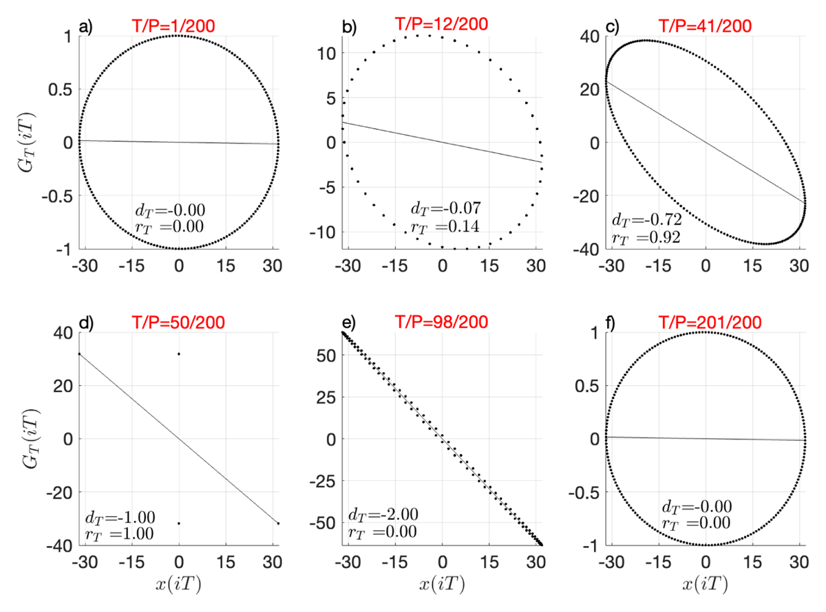
Figure 8
Same as Figure 2, but for the cosine model dx/dt = cos(2π t/P) with period P = 200 for six different values of T. Dots are the points (x(t), GT(t)) with t = iT, i = 0,1,… n, and n = 103. They overlap when the periods of (x(iT), GT(iT)), which vary with T, are shorter than n. Lines are regressions GT(iT) = cT+dT x(iT) obtained from the n points. Numbers listed are values of dT and with . Note that if T is a multiple of P/2, we have GT,iT = 0. Different from Figure 2, the symbol ^ is dropped, since for n that is a multiple of P, cT, dT, and do not change with increasing n.
Postulate II is also valid for the cosine model. The points (black dots in Figure 4), which can be calculated using the analytical expressions of GT(iT) and x(iT) with i=1,…, n, are located right on the corresponding fd-curve, which is indicated by the orange line in Figure 4a) and collapses to the black line in Figure 4b). Thus, the dissipating and fluctuating component of the integral forcing of a periodic solution are also related to each other via Eq. (12).
The situation is different for Postulate III. The general strengthening of dT with increasing T, which in this example can only occur in a non-monotonic manner, cannot be realized by the one-dimensional cosine model. dT, which is a periodic function of T, retains its overall strength with increasing T. The points or (black dots in Figure 4) swing with increasing T from the right end (where dT = 0) to the left end (where dT = –2) of the fd-curve and continue to swing with the same reach as T goes to infinity. No threshold of T exists such that for T larger than this threshold, GT(t) reduces to a forcing consisting of a dissipating component with dT = –1 and a white-noise like fluctuating component. Postulate III is not valid. The sinus solution at time t is always related to the sinus solution at time t+T later, independent of the value of T.
7 Conclusions
Consider a system described by a multi-dimensional state vector x, whose evolution is governed by a set of equations in form of dx/dt = F(x(t)) with x being a component of x and F = F (x(t)) being a deterministic function of x. When solving such a system at discrete time steps, the solution of x at a time step can become independent of the solution of x at a later time step, a behavior deemed as random. This paper examines how this randomness arises from internal dynamics represented by F. We do so by exploring the properties of the integral forcing Gτ,k, which equals the integral over F at τ time steps starting from the k-th time step. Gτ,k is responsible for the evolution of x from xk to xk+τ. The following conclusions are drawn.
First, for a system in equilibrium, the integral forcing Gτ,k consists of (apart from a constant cτ) a dissipating component dτxk with dτ < 0 and a fluctuating component fτ,k, and can be expressed as Gτ,k = cτ+dτ xk+fτ,k. This expression is in accordance with the idea behind the fluctuation – dissipation theorem that for a system in equilibrium, anything that generates fluctuations must also damp the fluctuations. The two components of Gτ,k are related to each other following the rule described by the fd-curve. There exists a threshold τ0 such that Gτ,k with τ > τ0 emerges as a unified forcing. The dissipating component of this forcing is characterized by dτ = –1, and the fluctuating component of this forcing behaves like a white noise, independent of τ, as long as τ > τ0, and no matter which component of x is considered.
Second, for τ > τ0, the state xk+τ, which is nominally produced by Gτ,k via xk+τ = xk+Gτ,k, equals then xk+τ = cτ+fτ,k, with fτ,k being a white-noise-like forcing. The series becomes random, since any one member in the series is independent of any other member of the series. This series is also irreversible, since a member xiτ is little by little canceled by the dissipation that emerges as soon as the system is integrated forward in time. By the time when the system is integrated over τ time steps to allow the emergence of Gτ,iτ, xiτ is completely canceled by the dissipating component of Gτ,iτ. xiτ+τ is generated by the fluctuating forcing of Gτ,iτ, which is independent of xiτ.
Third, while the damping in Fj represents a typically non-zero damping rate needed for counterbalancing the rate of external forcing, the dissipation in Gτ,k arises from actions completed over a time span of non-zero length. More precisely, these actions are interactions of xk with other components of x completed during the time span extending from time step k to time step k+τ–1. The number of these interactions inevitably goes to zero when the length of the time span goes to zero. It reaches a maximum, when the length of the time span equals τ0 time steps. Since the completion of these actions requires the passing of time, the resulting dissipation cannot be included in the differential forcing F.
Finally, being arising from interactions among components of x, randomness is a peculiar feature of a multi-dimensional system. The solution of a one-dimensional system cannot be random.
The above conclusions are drawn based on the integral forcing numerically obtained from the Lorenz’s 1963 model. Verifying them for high-dimensional systems requires great computational efforts. By suggesting that Gτ consists of a dissipating and a fluctuating component, we link the mechanism responsible for the emergence of randomness with the fluctuation-dissipation theorem known in statistical physics. By demonstrating that the dissipation in Gτ cannot be included in F but emerges as soon as the system is integrated forward in time, we identify the mechanism as resulting from interactions completed within a time span of non-zero length. When further verified, the idea behind the fluctuation and dissipation theorem should be considered as generally valid for multi-dimensional systems that are in equilibrium and governed by differential equations in form of dx/dt = F.
Appendix A: Calculation of intercept cτ, regression slope dτ and residual fτ,iτ
This appendix shows how the intercept cτ, the regression slope dτ, and the residual fτ,iτ (or the fluctuating component of Gτ,iτ) and its variance are calculated. Since Eq. (9) represents a regression of Gτ,iτ against xτ,i, we use the known result of least squared fitting and define
Given and , fτ,iτ is defines as
with variance
We use ^ to distinguish quantities obtained from a finite number n of data points from quantities obtained in the limit n → ∞:
and
For the Lorenz model, and (Figure 3) and (not shown) converge with increasing value of n.
Appendix B: Derivation of the fd-curve
This appendix derives the fd-curve that describes the relation between the dissipating and fluctuating component of an integral forcing Gτ,iτ with . We start from expressing Gτ,iτ in terms of intercept , regression slope and residual , defined using n data points along a solution, with n being finite, and proceed further by considering the limit n → ∞.
For , we rewrite Eq. (8) using Eq. (A3) as
We define the mean and the variance of the series {xiτ|i=1,…, n} by
and the mean of by
and the covariance between and xiτ by
where
Rearranging Eq. (B1) by expressing x(i+1)τ in terms of and xiτ in terms of through adding and subtracting , we find,
Squaring Eq. (B7) and applying to the result, we obtain after making use of ,
with
For a sufficiently large n, is well approximated by . Eq. (B8) reduces to
Figure B1 shows for the three Lorenz components and for τ = 2 and τ = 5000 respectively, how the three A-terms defined in Eq. (B9)–Eq. (B11) evolve with increasing number n of data points used for their calculations. A1 and A2 (first two rows) converge fast to zero with increasing n. A3 (bottom panel) is numerically not distinguishable from zero for all considered values of n. Similar behaviors are found for other values of τ, including τ = 1. The three A-terms in Eq. (B12) can hence be considered to be zero for for sufficiently large value of n. In the limit n → ∞, Eq. (B12) can, after making use of Eq. (A7) and
be rewritten as
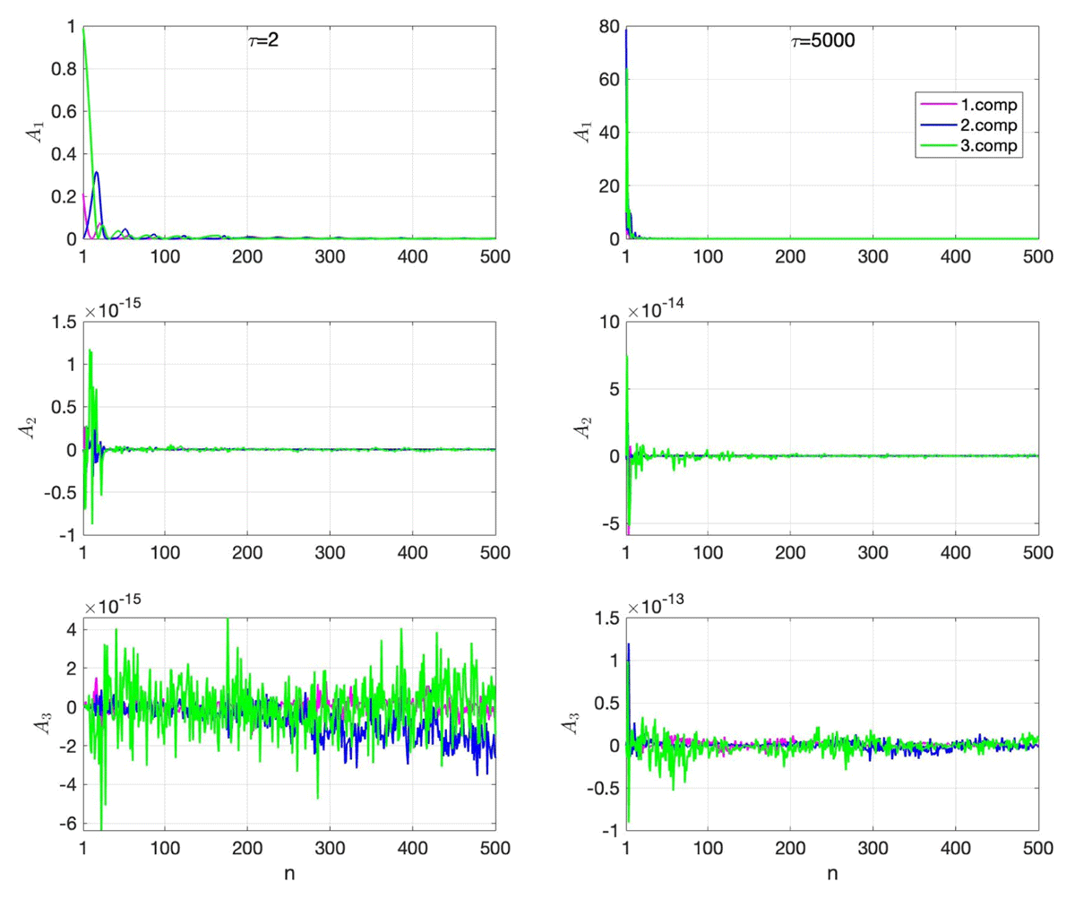
Figure B1
A1 (top), A2 (middle), and A3 (bottom) as functions of n, derived for the three Lorenz components (magenta, blue and green) and for τ = 2 (left) and τ = 5000 (right). n is the number of consecutive data points along a stationary solution used to calculate A1, A2 and A3.
That the limit Eq. (B13) is independent of τ can be easily demonstrated numerically.
Appendix C: Derivation of the relation between ρτ and dτ
This appendix establishes the relation between auto-correlation function ρτ of x and dτ associated with the integral forcing Gτ of x. For and the respective covariance function are defined by
where is defined in Eq. (B2). Multiplying Eq. (B7) by and applying (for its definition, see Eq. (B6)) to the result yields
where the equality is used. Since can be shown to be numerically not distinguishable from zero, similar to A3 discussed in Appendix B, we can set to zero. In the limit n → ∞, Eq. (C2) reduces then, after making use of Eq. (B13), to
Data Accessibility Statement
All data and subsequently the figures are generated by Matlab-scripts archived in the publication repository: https://hdl.handle.net/21.11116/0000-000D-C83B-0.
Acknowledgements
I thank Eduardo Zorita and Cathy Hohenegger who read an early version of this paper and provided suggestions extremely helpful for enhancing the accessibility of the paper. I am grateful to the anonymous reviewers (especially reviewer A) for their critical comments, which led to the reformulation of a few key aspects of the theory. I am also grateful to the Max-Planck Institute for Meteorology for the inspiring atmosphere. The discussion with my colleagues there helped to sharpen some of the arguments.
Competing Interests
The author has no competing interests to declare.