
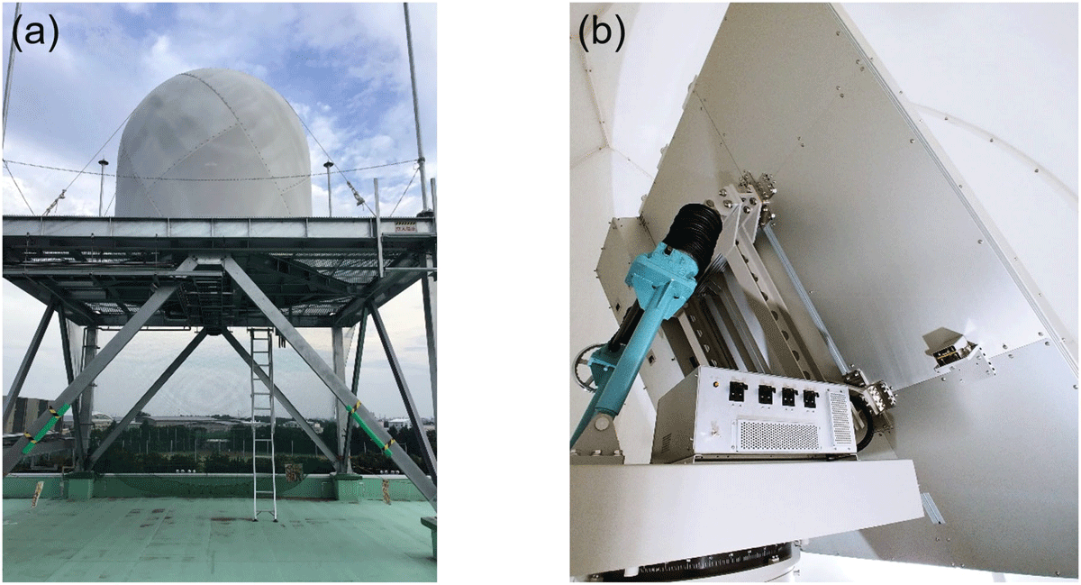
Figure 1
Photos of (a) the MP-PAWR and (b) the phased array antenna.
Table 1
Specification of the MP-PAWR.
| PARAMETERS | AUTO-01 | AUTO-02 |
|---|---|---|
| Antenna element | Dual-polarized patch antenna | |
| Frequency | 9425 MHz | |
| Azimuth resolution | 1.2 degree | |
| Elevation | 0.0~60.0 degrees 0.0~90.0 degrees | |
| Elevation resolution | 0.5~1.0 degrees | |
| Number of elevation | 77114 | |
| Observation radius | 80 km60 km | |
| Range resolution | 150 m75 m | |
| Time resolution for volume scan | 60 sec30 sec | |
| Pulse width | 1 μs (short)1 μs (short) | |
| 74 μs (long)48 μs (long) | ||
| Observation variables | Radar reflectivity (Z) | |
| Differential reflectivity (Zdr) | ||
| Differential phase (Φdp) | ||
| Specific differential phase (Kdp) | ||
| Doppler velocity (V) | ||
| Spectrum width (W) | ||
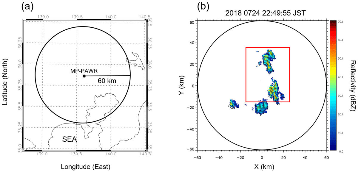
Figure 2
(a) Map of the MP-PAWR coverage (AUTO-02 mode) and (b) the observed Z field at 22:49:55 JST on July 24, 2018, which is an initialized time (t0) for all model forecasts. Here, Japan Standard Time (JST) = UTC + 9. In (b), the red box indicates the experiment domain of the CNN models (40 × 50 km) and the arrows that denote motion vectors are obtained from the optical flow method.
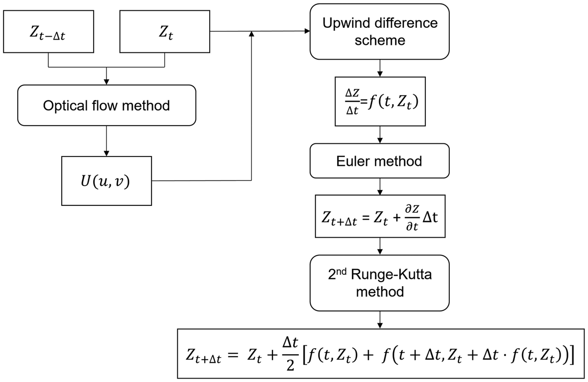
Figure 3
Flowchart of the AFM nowcast.
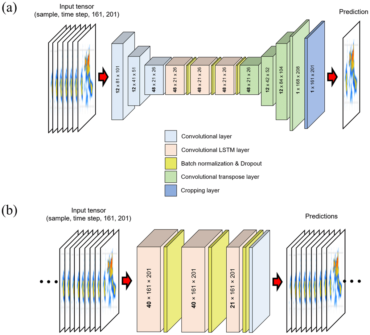
Figure 4
Schematics of (a) the EDM and (b) the CLM architecture. A bolded number indicates the number of filters used in the convolutional LSTM layer. In this study, the number of time steps for the EDM is 7 and for the CLM is 20. The activation function of ReLU was used in all the layers of convolution.
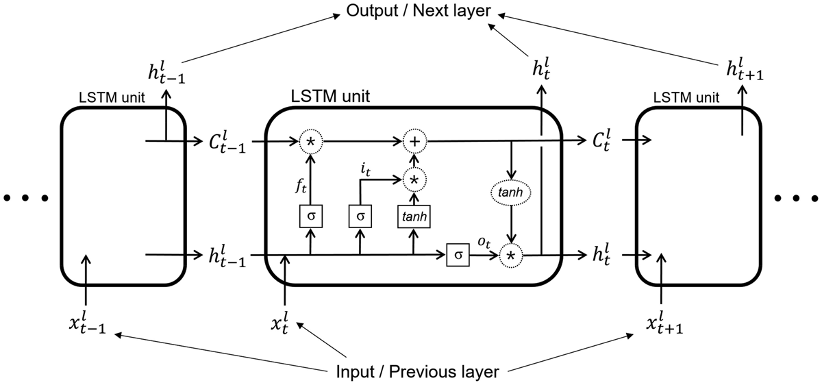
Figure 5
Schematic of an LSTM layer with regard to Eq. (5). The superscript l is the number of layer and the subscript t is time of sequences. Please refer to the text for more details.
Table 2
A summary of statistics of each model with lead time.
| LEAD TIME | MODEL | CORRELATION COEFFICIENT | MEAN BIAS | ROOT MEAN SQUARED ERROR | STANDARD DEVIATION |
|---|---|---|---|---|---|
| 2.5 min | CLM | 0.88 | –0.37 | 6.84 | 6.83 |
| EDM | 0.73 | –2.4 | 8.92 | 8.6 | |
| AFM | 0.87 | 0.9 | 7.0 | 6.94 | |
| 5 min | CLM | 0.69 | 0.3 | 9.51 | 9.51 |
| EDM | 0.61 | –3.27 | 10.55 | 10.03 | |
| AFM | 0.65 | 0.86 | 10.56 | 10.53 | |
| 7.5 min | CLM | 0.58 | –0.22 | 10.41 | 10.41 |
| EDM | 0.51 | –1.22 | 10.77 | 10.71 | |
| AFM | 0.46 | 2.01 | 12.63 | 12.47 | |
| 10 min | CLM | 0.56 | –0.74 | 8.96 | 8.93 |
| EDM | 0.48 | –2.08 | 11.66 | 11.47 | |
| AFM | 0.36 | 2.28 | 14.05 | 13.86 |
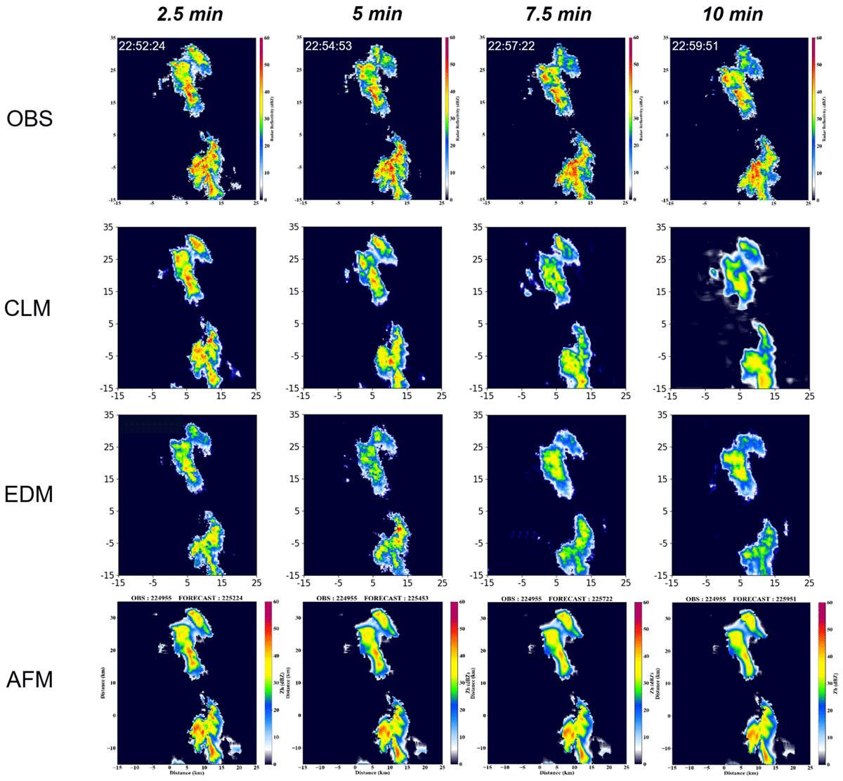
Figure 6
Comparison of the observed (OBS) and predicted Z fields from the CLM, EDM, and AFM with lead time.
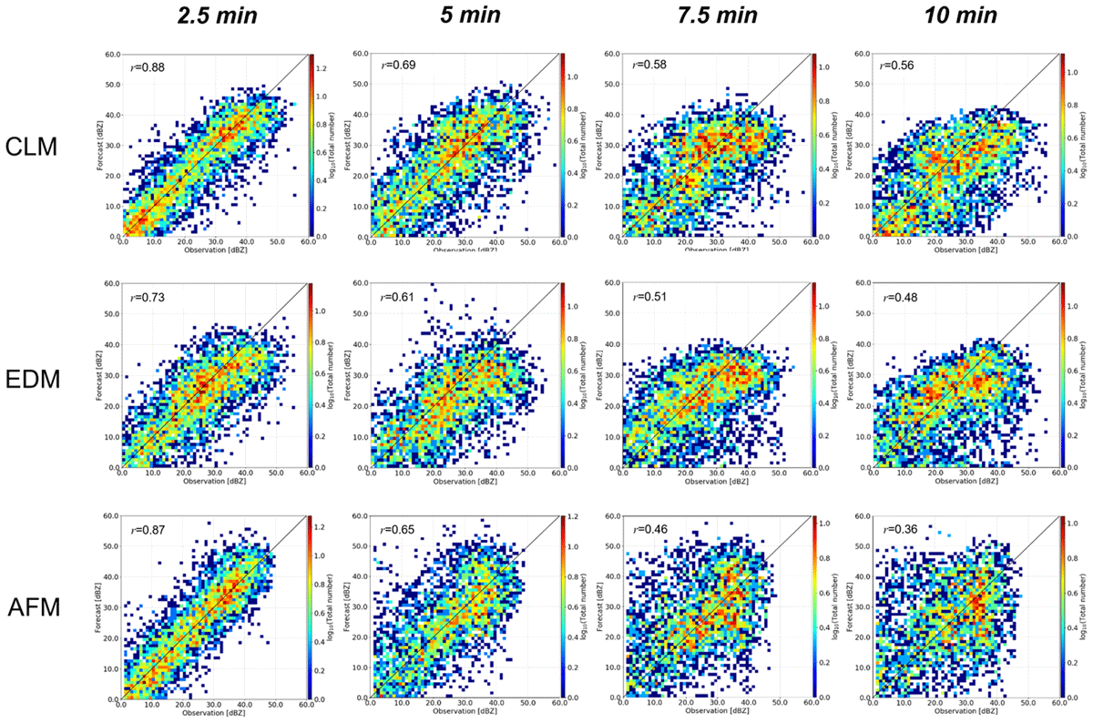
Figure 7
Scatterplots with correlation coefficients between observations and forecasts with lead time for the total rain area category of Z > 10 dBZ.
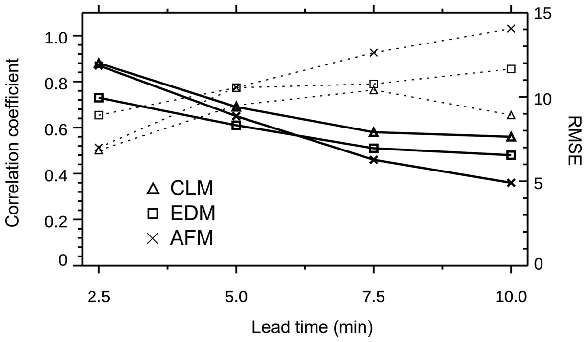
Figure 8
Time series of the correlation coefficients (solid) and RMSEs (dotted) of the CLM, EDM, and AFM for the total rain area of Z > 10 dBZ. A legend for the symbols of the models is shown in the left-bottom corner.
Table 3
A summary of the nowcasting metrics with lead time for the two categories of Z >10 dBZ and Z > 35 dBZ (in the bracket).
| LEAD TIME | MODEL | POD | FAR | CSI (THREAT SCORE) |
|---|---|---|---|---|
| 2.5 min | CLM | 0.91 (0.69) | 0.08 (0.27) | 0.85 (0.55) |
| EDM | 0.88 (0.35) | 0.07 (0.34) | 0.83 (0.30) | |
| AFM | 0.91 (0.76) | 0.09 (0.33) | 0.83 (0.55) | |
| Persistence | 0.88 (0.62) | 0.14 (0.35) | 0.78 (0.46) | |
| 5 min | CLM | 0.90 (0.52) | 0.14 (0.46) | 0.78 (0.36) |
| EDM | 0.84 (0.17) | 0.10 (0.49) | 0.77 (0.15) | |
| AFM | 0.87 (0.49) | 0.15 (0.51) | 0.76 (0.32) | |
| Persistence | 0.82 (0.43) | 0.20 (0.62) | 0.68 (0.25) | |
| 7.5 min | CLM | 0.87 (0.29) | 0.17 (0.49) | 0.74 (0.23) |
| EDM | 0.84 (0.10) | 0.17 (0.62) | 0.72 (0.09) | |
| AFM | 0.87 (0.40) | 0.20 (0.64) | 0.71 (0.23) | |
| Persistence | 0.76 (0.35) | 0.23 (0.66) | 0.62 (0.21) | |
| 10 min | CLM | 0.81 (0.21) | 0.17 (0.42) | 0.70 (0.16) |
| EDM | 0.81 (0.07) | 0.17 (0.58) | 0.69 (0.07) | |
| AFM | 0.85 (0.35) | 0.25 (0.70) | 0.66 (0.19) | |
| Persistence | 0.71 (0.31) | 0.27 (0.71) | 0.56 (0.17) |
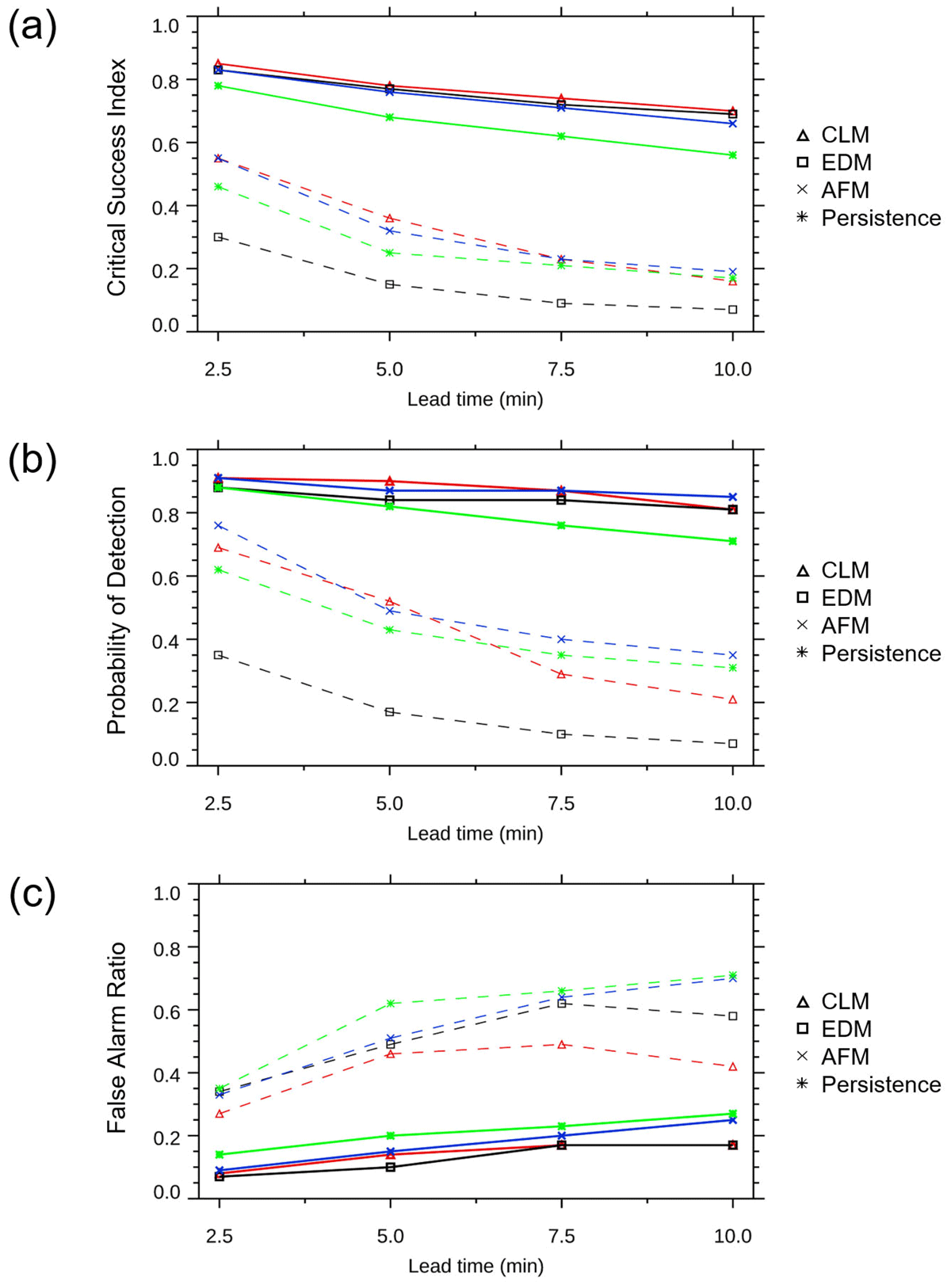
Figure 9
Time series of the scores of (a) CSI, (b) POD, and (c) FAR from the CLM, EDM, AFM, and persistence method. The solid line is for the total rain area and the dashed for the convective rain area. The CLM is in red, the EDM in black, the AFM in blue, and the persistence method in green.