
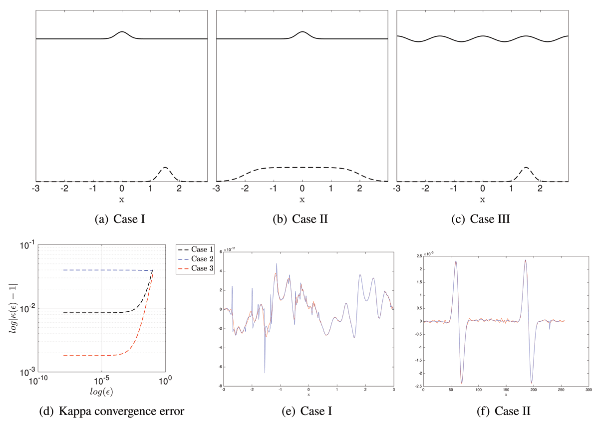
Figure 1
(a)–(c): The three test cases for bathymetry β(x) (dashed line) and surface wave initial conditions ϕ(x) (solid line) for the data assimilation. The surface wave initial conditions , bathymetry , and average depth H are not to scale in these diagrams, as was restricted to 1% of across most of the numerical analyses, and β = 0.1. (d): The log error in the convergence of the kappa test in (3.1), to verify the numerical calculation of the Hessian. (e) and (f): ν (red) and (blue) for cases I and II where ν is the solution of ν = found using the matlab linear solver bicgstabl.
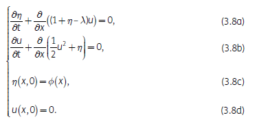
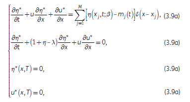
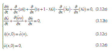
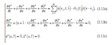
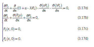
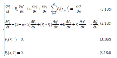
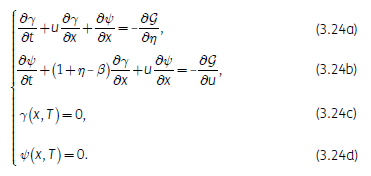
Algorithm 1
Calculation of Second Order Adjoint Sensitivity ∂m for Bathymetry Assimilation.
| 1: | Define , where γ is the solution of (3.24). |
| 2: | Solve ν = for ν, where is the Hessian operator acting on ν, and is the forcing term defined by (3.2) in step 1. |
| 3: | Solve the system (3.17) by substituting the control variable P5(x) with ν (as found in step 2) to find the adjoint variable P3(x, t). |
| 4: | Define , where P3 has been sampled at the locations of the observation points {xj}. |
Table 1
Cases considered for data assimilation algorithm, and comparison of the relative L2 reconstruction error (4.2) in the bathymetry as shown in Figure 4 of Khan and Kevlahan (2021), and the time integrated sensitivity of the surface wave error to the observations.
| CASE | BATHYMETRY | INITIAL CONDITIONS | ERROR | SENSITIVITY |
|---|---|---|---|---|
| I | Gaussian | Gaussian | 𝒪(10–3) | 𝒪(10–9) |
| II | Sandbar | Gaussian | 𝒪(10–2) | 𝒪(10–5) |
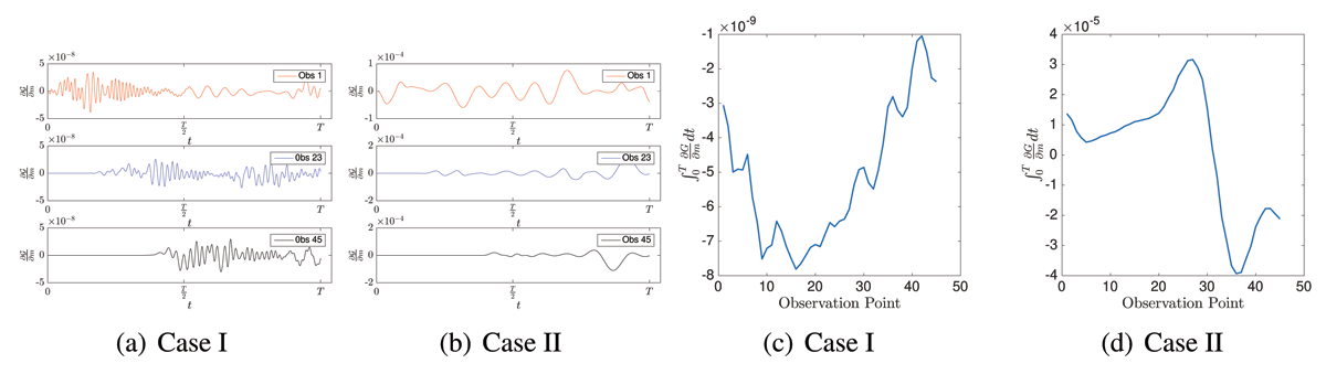
Figure 2
(a, b) The sensitivity d/dm as a function of time (with final time t = T), for assimilation results for Case I. There are Nobs = 45 observations, equidistantly spaced with Δx = 0.06 and with the first point at 0.1L. Results show d/dm at three distinct observation points mj, where j = 1 (first observation), (the median observation), and Nobs (the last observation). (c, d) The time integrated sensitivity at each observation point.
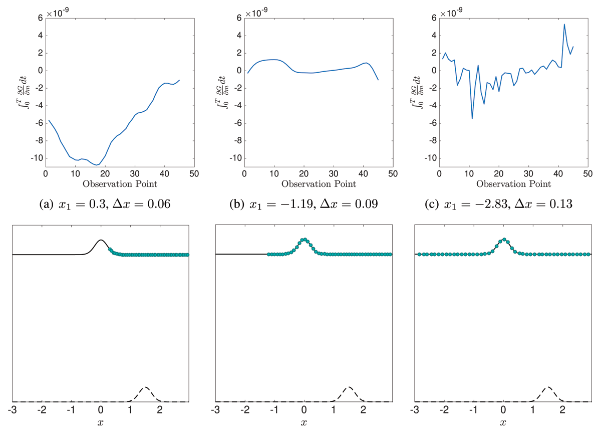
Figure 3
Case I: The time integrated sensitivity of the surface wave error as the location of the first observation point is varied such that the observation points cover a greater proportion of the domain and the initial conditions support.
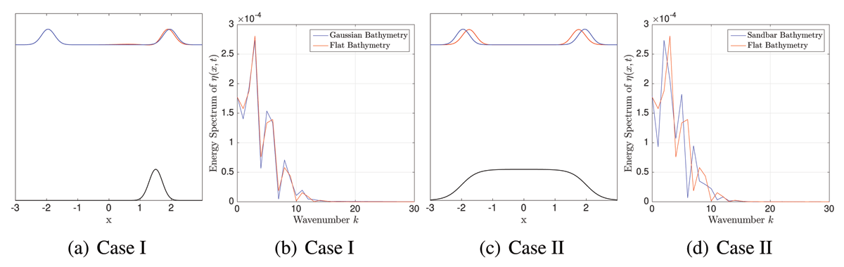
Figure 4
(a, c) The surface wave at t = 1.95 given a flat bathymetry (red), and non-zero bathymetry (blue). The amplitudes of bathymetry and initial condition are not to scale, however the location is accurately represented. (b, d) Spectrum of the surface wave given a flat bathymetry and non-zero bathymetry for Cases I and II respectively.
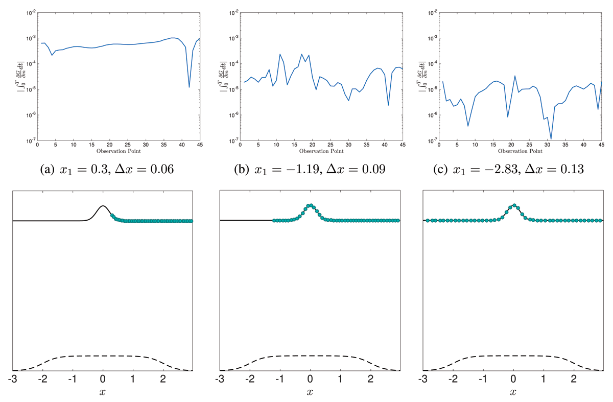
Figure 5
Case II: the absolute time integrated sensitivity of the surface wave error as the location of the first observation point is varied such that the observation points cover a greater proportion of the domain and the initial conditions support.
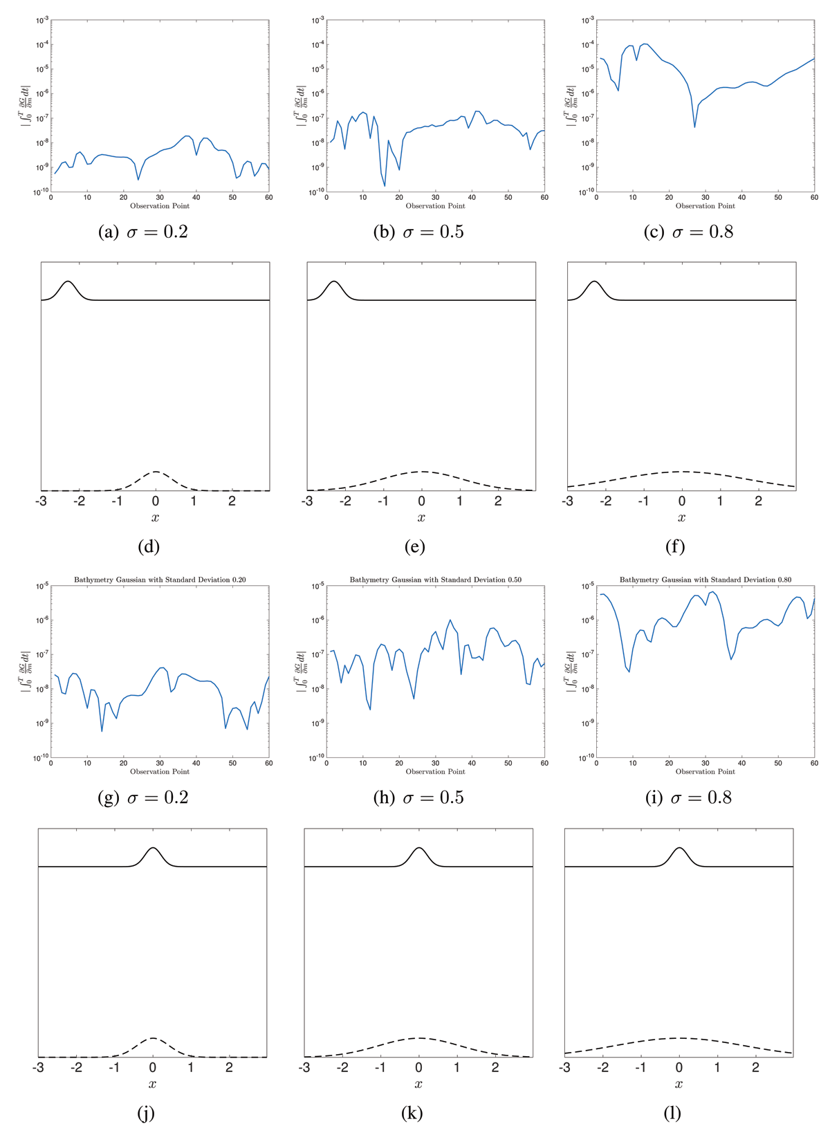
Figure 6
The absolute time integrated sensitivity as the standard deviation of the bathymetry Gaussian is increased. (a–f) show results with the initial condition to the right of the bathymetry, like Case I. (g–l) show results with both the initial conditions and bathymetry centred at x = 0, like Case II.
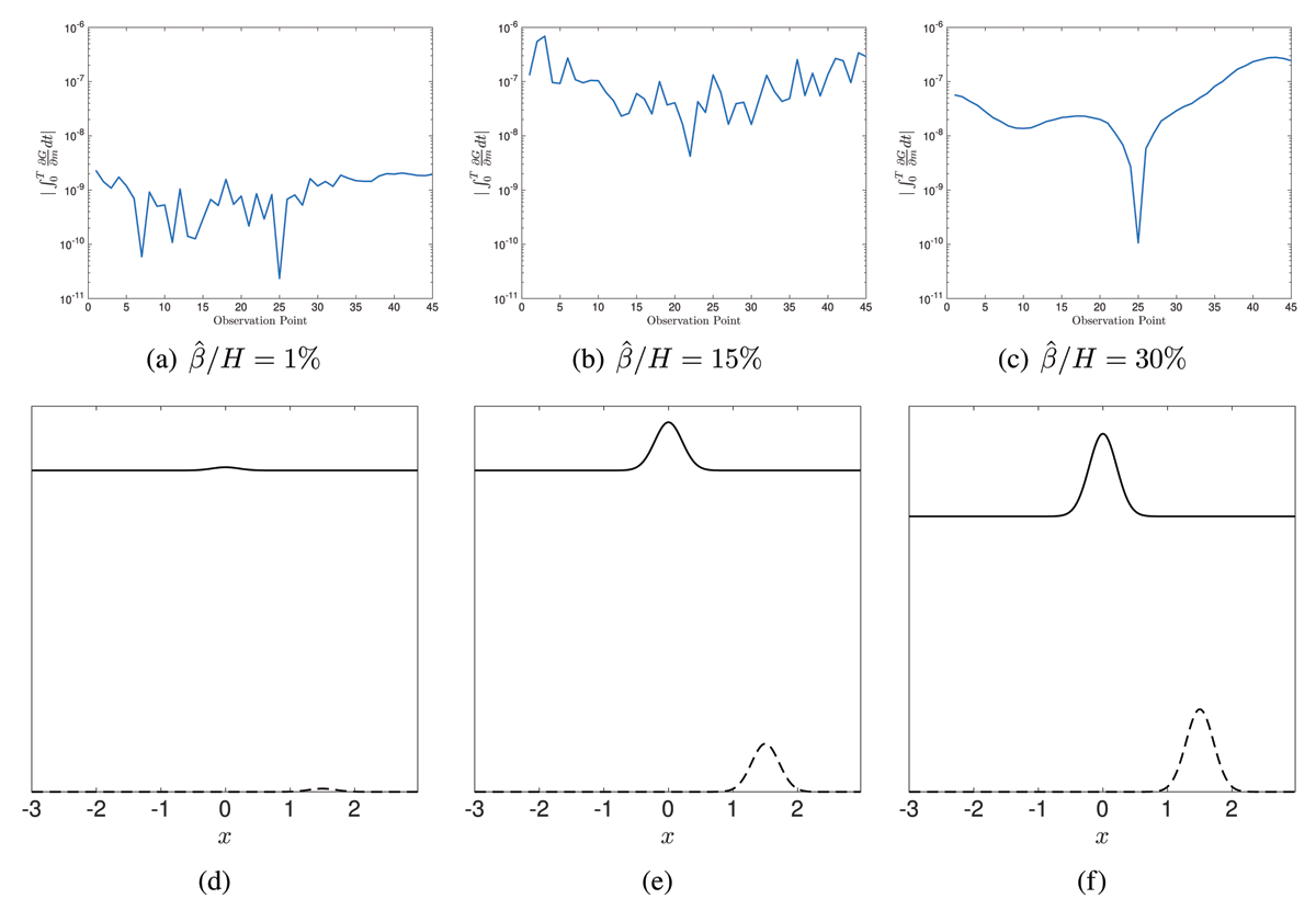
Figure 7
Case I: Absolute time integrated sensitivity as the relative amplitude of the bathymetry is increased.
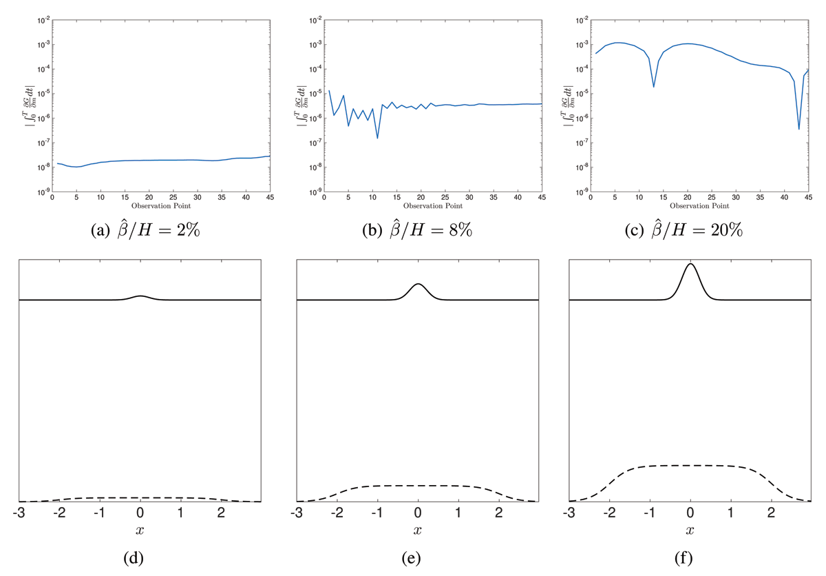
Figure 8
Case II: absolute time integrated sensitivity as the relative amplitude of the bathymetry is increased.