
1 Introduction
The description of cloud processes and precipitation formation remains challenging in atmospheric modeling. Microphysical processes influence moisture distribution in the atmosphere and the occurrence of clouds. They also contribute significantly to the energy cycle via water phase changes by latent heat sink/release and also via the interaction of clouds with radiative transfer. Such processes are multi-scale, going from large-scale stratiform processes to local intensive convective storms and showers.
High precipitation accumulations can lead to floods, which are among the most severe weather threats. Precipitation distribution is also a key parameter for the climate. Therefore, it is important to continue improving cloud and precipitation schemes in numerical weather prediction (NWP) and climate models, which is a demanding task. Besides their growing physical complexity, schemes need to stay computationally efficient by using a numerically robust treatment of water phase changes and sedimentation of hydrometeors. In addition, they need to also cope with the above-mentioned multi-scale character of conditions leading to precipitation formation.
Over the past three decades, several prognostic bulk microphysics schemes were developed with different degrees of complexity. The number of hydrometeors simulated prognostically in these schemes usually ranges from three to six. Certain schemes operate with three prognostic hydrometeors: cloud water, rain, and one shared ice category among all ice particles (Wilson and Ballard (1999), or a much more sophisticated Morrison and Milbrandt (2015), which uses multiple ice prognostics making the scheme much more physically accurate). Some schemes simulate four hydrometeors prognostically (Delanoë et al. 2011; Lopez 2002); namely, cloud water, rain, cloud ice, and snow, making such schemes two-ice. More complex schemes have five prognostic hydrometeors (Field et al. 2023; Hong and Lim 2006; Pinty and Jabouille 1998; Thompson et al. 2004) with graupel being the additional third ice particle. Some schemes add hail (Seifert and Beheng 2006; Vié et al. 2016). Currently, most operationally used schemes in NWP simulate four or five hydrometeors prognostically. Often, the mass of hydrometeors is the only prognostic variable (Hong and Lim 2006; Lopez 2002; Pinty and Jabouille 1998; Wilson and Ballard 1999). Such schemes are called single-moment. Alternatively, double-moment schemes predict not only the mass of hydrometeors but also their number concentration (Field et al. 2023; Seifert and Beheng 2006; Thompson and Eidhammer 2014).
A single-moment microphysics scheme with four prognostic hydrometeors is also used in ALARO, which is one of the three canonical model configurations of the ALADIN System (Termonia et al. 2018). The ALARO scheme is unique in treating the multi-scale problem by a single call of microphysics, which is included in the sequence of calls of the deep convection parameterization 3MT (Gerard et al. 2009). The microphysics scheme then operates upon the sum of convective and stratiform (grid-scale) condensates, blurring their origin. Usually, the microphysics is treated separately for convective and grid-scale (working upon condensates from the cloud scheme) parts (Gerard 2015). The suitability of this approach for horizontal resolutions ranging from 1 to 16 km was demonstrated by Field et al. (2017). Moreover, the microphysics scheme can also be used for the stratiform part only.
The two-ice ALARO microphysics scheme became operational at the Czech Hydrometeorological Institute in 2007, first operating only upon grid-scale condensates from the cloud scheme and since 2008 in the sequence of calls of the deep convection parameterization 3MT (Gerard et al. 2009).
In this article, we describe an enhancement of the microphysics scheme used in ALARO from the two-ice to the three-ice scheme by adding graupel. The major challenge of graupel parameterization is to make the parameterization physically realistic because graupel acquires many shapes and densities (Heymsfield et al. 2018). This results in many proposed parameterizations of its fall speeds and shapes (Vázquez-Martín, Kuhn, and Eliasson 2021; Locatelli and Hobbs 1974). The selected parameters for simulating graupel were shown to have a significant impact on precipitation intensity in heavy rainfall events (Li et al. 2019) and on a bow echo simulation (Adams-Selin, van den Heever, and Johnson 2013).
Furthermore, microphysical process conversion rates are often highly uncertain (Morrison et al. 2020). This leads to multiple formulations of the same process across microphysics schemes, giving us the possibility to test its various parameterizations in our framework. In the second part of this article, some enhancements of these parameterization options for microphysical processes are introduced. This should reduce known deficiencies of the current microphysics scheme such as positive precipitation bias by introducing more physically based parameterizations of microphysical processes and adjusting their coefficients.
The structure of the article is as follows: The ALARO microphysics scheme, which is further developed in this article, is described in Section 2. The introduction of graupel in the microphysics scheme and adjusting its parameters, together with a revision of selected microphysics processes of all hydrometeors, is described in Section 3. Methods used for validation are described in Section 4. Results are provided in Section 5, leading to their discussion and conclusion in Section 6.
2 Two-Ice Microphysics Scheme
The microphysics scheme in ALARO is designed for use in a wide range of resolutions, which is ensured by two closely related specific features. First, if deep convection is parameterized, the microphysics is embedded in the framework of the deep convection parameterization 3MT, operating upon the sum of condensates from the cloud scheme and the updraft from the deep convection scheme. Second, a specific geometry is employed, dividing the gridbox into four parts, accounting for the sub-grid variability of clouds and precipitation (Gerard et al. 2009). A hypothesis for cloud overlap must be employed, which is in the ALARO microphysics maximum-random, i.e. maximum overlap between clouds in adjacent layers and random overlap between clouds with clear-sky layers in between.
Because of the vertical overlap of clouds and precipitation in the four gridbox parts, the calculation is organized in a vertical loop going from the top of the atmosphere to the ground. Microphysical processes are calculated for each model layer. When passing from one layer to the next, areas of non-seeded (by precipitation) cloudy, non-seeded clear-sky, seeded cloudy, and seeded clear-sky are computed. Autoconversion and collection occur only in cloudy parts. Evaporation occurs only in non-cloudy parts and melting occurs in all parts. The precipitation flux is computed for every part separately. The numerical stability of the sedimentation of precipitation in this loop is ensured by a statistical treatment (Geleyn et al. 2008).
As stated in Termonia et al. (2018), the included microphysical processes in the two-ice microphysics scheme in ALARO are inspired by Lopez (2002). The individual parameterization choices are described in Catry (2006), from which the current two-ice scheme differs only in some details.
The scheme is single-moment with five prognostic water species: water vapor, cloud water, cloud ice, rain, and snow, with their mass fractions qv, ql, qi, qr, and qs, respectively. In addition, the mass fraction of graupel can be diagnostically obtained within the snow category. Its mass fraction is obtained based on ratios of microphysics process fluxes, with the primal source of graupel being the WBF process. Such diagnostic graupel affects the fall speed and collection rates of the mixed snow category and is used for a hail diagnostic.
Figure 1 shows microphysical processes simulated by the two-ice scheme. The source terms of rain are autoconversion from cloud water and melting of snow. The collection of cloud water and cloud ice contributes to its growth. Its sink terms are evaporation, freezing to snow, and sedimentation. Although cloud ice is collected into the rain category, the latent heat influence on temperature raises the probability of rain freezing in the same time-step as the collection computation precedes the freezing computation. Snow is produced by autoconversion from cloud ice, the Wegener-Bergeron-Findeisen (WBF) process depleting the cloud water (Van der Hage 1995), and freezing of rain. Snow also collects cloud water (riming) and cloud ice. Sink terms of snow are sublimation, melting, and sedimentation.
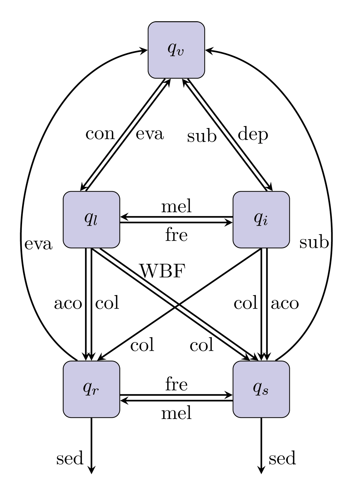
Figure 1
Illustration of microphysical processes in the two-ice scheme. Aco is autoconversion, col collection, con condensation, dep deposition, eva evaporation, fre freezing, mel melting, sed sedimentation, sub sublimation, and WBF is the WBF process.
The current ALARO microphysics scheme contains two enhancements with respect to Catry (2006). The first one is using a modification of the intercept parameter of the negative exponential distribution proposed by Abel and Boutle (2012) (see Appendix A5) instead of the Marshall-Palmer distribution (Marshall and Palmer 1948).
The other enhancement is the parameterization of the WBF process based on Van der Hage (1995), which is treated as a special case of autoconversion from cloud water to snow if enough cloud ice is present (Gerard et al. 2009). The short phase of wet ice crystals is bypassed as the rapid growth of the ice crystal and its quick conversion into a precipitating category is assumed (Brožková 2014).
Autoconversion for all species, including the WBF process, is parameterized following Sundqvist (1978), described in detail in Appendix A1.
Collection is handled by the continuous growth model (Appendix A2). Only cloud particles can be collected by precipitating particles. Collection always leads to the growth of the precipitating category, and the precipitating particle never changes its category. Thus, there are no three-particle interactions. The only difference between the collection efficiency used for collecting cloud water and cloud ice is that the collection of cloud ice is less efficient for lower temperatures regardless of the species of the collector.
A Kessler-type evaporation parameterization (detailed in Appendix A3) is used for all precipitating hydrometeors. This parameterization is based on the data from the Smithsonian meteorological tables (List et al. 1951) following Kinzer and Gunn (1951) and was derived for raindrops only. Consequently, sublimation rates of snow must be determined. Two competing processes come under consideration. A less dense particle evaporates quicker since the ratio of the area to the volume of the particle is higher than for denser particles. Contrary, such a particle also falls slower, so its ventilation is less. Because these processes are assumed to cancel each other out, the coefficients of the Kessler-type evaporation parameterization of rain and snow are assumed equal except for the consideration of the ratio between the specific latent heat of sublimation to the specific latent heat of evaporation, which lowers the sublimation rates for ice hydrometeors (Geleyn et al. 2011). This hypothesis only holds when the Marshall-Palmer distribution is used for rain. For the modified intercept parameter by Abel and Boutle, (2012) the equation for evaporation is adjusted, while the sublimation rates of snow are unchanged.
Melting is parameterized by a similar formula as evaporation, with only the ratio of the specific heat of melting to the heat capacity of water is taken into consideration, as described in Appendix A4.
The model configuration using this scheme is denoted by EMP0 in the validation part.
3 New Three-Ice Microphysics Scheme
3.1 Introduction of prognostic graupel
Graupel is introduced to the scheme as a third precipitating hydrometeor with its mass fraction qg. Figure 2 illustrates the organization of the resulting new three-ice scheme.
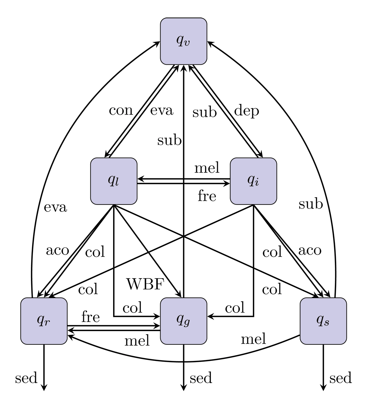
Figure 2
Same as Figure 1 but for the three-ice scheme.
Keeping consistency with the former diagnostic graupel, the WBF process produces prognostic graupel. The rationale behind this choice is to bypass the short stage of cloud ice existence before it grows to a precipitating category. Besides that, graupel is also produced by the freezing of rain. Both processes now contribute to the growth of graupel instead of snow. Graupel collects cloud water and cloud ice. Sink terms of graupel are sublimation, melting, and sedimentation.
On top of that, a set of choices for the parameterization of prognostic graupel was made. First, the Marshall-Palmer distribution with a fixed intercept parameter is chosen, which is a widely used option (Locatelli and Hobbs 1974; Rutledge and Hobbs 1984; Thompson et al. 2004). The selected intercept parameter follows Rutledge and Hobbs (1984), having a value of N0,g = 4 · 106 m–4.
Second, the parameterized terminal fall speeds of graupel particles across microphysics schemes are usually lower than that of rain and higher than that of snow if the precipitation flux is identical (Locatelli and Hobbs 1974; Hong and Lim 2006; Pinty and Jabouille 1998). After testing multiple options, the most suitable formulation according to the performance on standard atmospheric scores and other validation metrics appears to be w(D) = 124 · D0.66 (ρ0/ρa)0.4, where D is the particle diameter, ρa is the density of air, and ρ0 is the reference air density. This formula follows Locatelli and Hobbs (1974), but a density dependency was added similarly to the simulated fall speeds of other hydrometeors in the scheme.
Third, the shapes of graupel particles vary significantly. Nonetheless, handling such a variety of shapes in an NWP model is not feasible. Thus, it is common across microphysics schemes to consider graupel as spherical (Field et al. 2023; Hong and Lim 2006; Ikuta et al. 2021; Thompson et al. 2008) or with a mass-size relation using the power of diameter close to three (Pinty and Jabouille 1998; Vié et al. 2016) assuming a slightly non-spherical shape. We stay with the simple assumption of a spherical shape.
Fourth, the density of graupel heavily changes during its lifetime due to ambient conditions (Heymsfield et al. 2018), so the uncertainty of the graupel density is high. The typical fixed values of graupel density range between 300 and 500 kg∙m–3 across microphysics schemes (Field et al. 2023; Hong and Lim 2006; Thompson et al. 2008). We assume a constant density of 400 kg∙m–3, which should well represent its average density (Heymsfield et al. 2018).
Regarding microphysics processes, the parameters of the WBF process follow the recommended values by Geleyn et al. (2007), detailed in Appendix A1. The equation for collection was derived according to the new parameters for graupel using a collection efficiency of Eg = 0.15, a value in between the ones of rain (Er = 0.2) and snow (Es = 0.1). Formulae for the Kessler-type of sublimation and melting are inherited from snow as graupel is also an ice hydrometeor.
The complete set of parameters for graupel is listed in Table 1. This model configuration is denoted by EMP1.
Table 1
The proposed set of parameters for graupel. The diameter of a graupel particle is denoted by D and its density by ρg.
| PARAMETER | PROPOSED VALUE |
|---|---|
| fall speed relation | |
| density of graupel | ρg = 400 kg · m–3 |
| size distribution | Ng(D) = N0,ge–λD |
| intercept parameter | N0,g = 4 · 106 m–4 |
| mass-size relation | |
| collection efficiency | |
| autoconversion coefficient | kg = 10–3 s–1 |
| first WBF coefficient | |
| second WBF coefficient |
3.2 New options and adjustments of microphysical processes
The introduction of prognostic graupel improved the model results. However, as discussed in Section 5, some known issues remain, such as positive precipitation bias, which is more pronounced in autumn and winter, overestimated precipitation maxima in convective storms, or weak precipitation shadow behind mountain ranges. To reduce these imperfections, parameters of selected microphysical processes are adjusted, and new options in the parameterizations of autoconversion and evaporation are introduced in this section. Their summary is listed in Table 2.
Table 2
Differences between the microphysical choices made in EMP1 and EMP2.
| PROCESS | EMP1 | EMP2 |
|---|---|---|
| evaporation parameterization | Kessler | Lopez |
| kr (Equation A1) | 5∙10–4 | 8∙10–4 |
| (Equation A1) | 3∙10–4 | 4∙10–4 |
| ks (Equation A3) | 2∙10–3 | 10–3 |
| cpart (Equation A13) | 1 | 0.75 |
3.2.1 Autoconversion
As mentioned in Section 2, ALARO uses the Sundqvist-type of autoconversion. We aim to revise the set of its parameters. The formula for the Sundqvist-type of autoconversion can be written as
where kr/s are autoconversion coefficients, and is the parameter of the threshold function. Unlike is temperature dependent. As a new option, its value can be computed following Chaboureau and Pinty (2006) as:
where Tt is the temperature of the triple point of water. This formula was derived using the satellite observations of cirri in the tropical areas. However, it did not prove to be suitable for mid-latitude winter cases due to a reduction in middle and high cloud cover. The reason is that snow transfers water (as a substance) to lower model levels, reducing relative humidity at the level of snow origin. Thus, Equation (2) is not retained in the presented experiments, and we stay with Equation (A2).
The value of ks is also temperature dependent as . The coefficient of ks,0 was lowered from 2 · 10–3 s–1 to 10–3 s–1. This adjustment raises the amount of cloud ice in cumulonimbus anvils, which was previously found to be too low (Sokol et al. 2021).
Regarding the autoconversion to rain, the value of kr in Equation (1) was increased from 5 · 10–4 s–1 to 8 · 10–4 s–1 and was raised from 3∙10–4 to 4∙10–4 kg∙kg–1. The latter should slightly reduce the current positive bias of precipitation accumulation in autumn stratus or stratocumulus periods when precipitation accumulations are low. Under such conditions, the production of rain is more sensitive to the threshold value than to the autoconversion coefficient kr as the amount of ql of slightly precipitating strati and stratocumuli is close to this threshold in the model. On the other hand, rain production in cumulonimbi is more sensitive to the autoconversion coefficient kr as is exceeded significantly.
3.2.2 Evaporation
As mentioned in Section 2, ALARO employs the Kessler-type evaporation parameterization. However, the Kessler-type evaporation parameterizations were found to produce too low evaporation rates (Ghosh and Jonas 1998). It is also possible to use another evaporation scheme following Lopez (2002) as a more physically based alternative. The Lopez scheme was extended for graupel and adjusted for the set of parameters used for rain in ALARO.
The equation for evaporation of a hydrometeor j is written as
where RH,l/i is the relative humidity with respect to water or ice, fc cloud fraction, ρa density of air, p pressure, Lv/s latent heat of evaporation/sublimation, Kt conductivity of air, T temperature, χ diffusivity of water vapor in the air, the saturation water vapor pressure over the phase of the hydrometor, and finally Ck (k ∈ {1,2,3,4}) are coefficients for which the values are listed in Table 3. Figure 3 shows evaporation and sublimation rates of all precipitating hydrometeors.
Table 3
List of parameters used in the evaporation parameterization of Equation (3). Coefficients for the new graupel parameterization are listed.
| COEFFICIENT | RAIN | SNOW | GRAUPEL |
|---|---|---|---|
| C1 | 2.2295 | 1227 | 230 |
| C2 | –1/9 | 2/3 | 0.5 |
| C3 | 8.738 | 2373.7 | 149 |
| C4 | 0.3807 | 1 | 0.7075 |
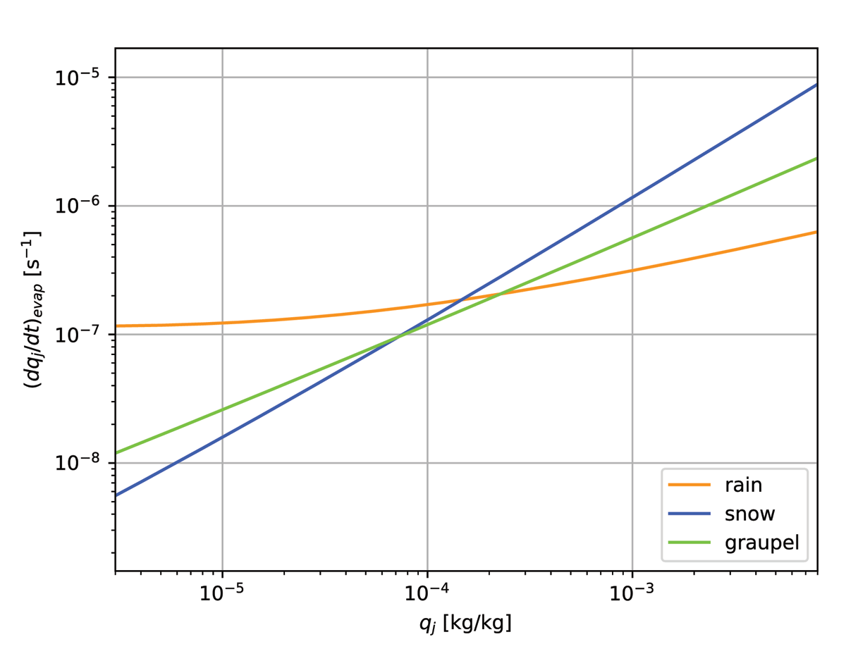
Figure 3
Dependency of the evaporation rates on the mass fraction of rain (orange), snow (blue), and graupel (green) at p = 100000 Pa, T = 273.15 K, and RH = 90% using the Lopez evaporation parameterization.
Since the evaporation parameterization following Lopez (2002) should deliver higher evaporation rates, a reduction in precipitation accumulations is expected.
However, this parameterization did not improve the typical atmospheric scores. Mainly the random error of wind speed was worsened due to too high evaporation rates near the surface (not shown). In order to dampen this effect, the evaporation rates given by Equation (3) are reduced as
where cj is a constant greater than zero, which limits the maximum evaporation rate for a given hydrometeor. The summation is taken over the uncorrected evaporation rates of all hydrometeors. We use this reduction only for rain with its constant cr = 7 ∙ 10–7 s–1. Its effect on lowering rain evaporation rates is shown in Figure 4.
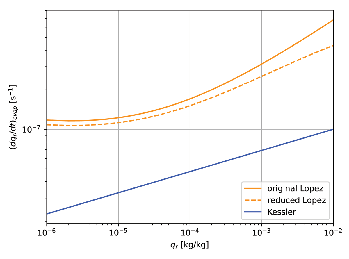
Figure 4
Dependency of the evaporation rates of rain on its mass fraction at p = 100000 Pa, T = 273.15 K, and RH = 90%. The evaporation rates of rain from the Lopez evaporation parameterization (Equation (3)) are in solid orange. Rain evaporation rates with the reduction of evaporation following Equation (4) are in dashed orange, coefficient cr = 7∙10–7 s–1. For comparison, the original Kessler scheme for rain is also shown (blue).
3.2.3 Further changes
In addition, the ice fraction in the split between cloud ice and cloud water in the thermodynamical adjustment was raised. On top of that, parameters of the cloud cover parameterization in the radiation scheme were adjusted to compensate for the increased cloud cover due to higher relative humidity caused by the Lopez evaporation scheme. First, the vertical profile of the critical relative humidity is more restrictive, requiring higher relative humidity to produce clouds. Second, the decorrelation length of the exponential-maximum-random cloud overlap used in the radiation scheme has a more distinct yearly cycle. The exponential-maximum-random cloud overlap introduces some decorrelation for cloud overlap in adjacent layers. The decorrelation length then describes where the maximum overlap becomes random.
The model configuration with the above-proposed modifications, except for the ice-to-snow autoconversion threshold described by Equation (2), is later denoted by EMP2.
4 Experimental Design and Methods
4.1 Tested configurations and periods
All tests were performed using the canonical model configuration ALARO of the ALADIN system (Termonia et al. 2018). The operational model configuration of the Czech Hydrometeorological Institute (Brožková et al. 2019) was used for validation.
The model domain, shown in Figure 5, consists of 1069 × 853 grid points with a resolution of 2.325 km in the Lambert conformal conic (LCC) map projection, onto which the domain is projected, and 87 vertical levels. The time-step is 90 s.
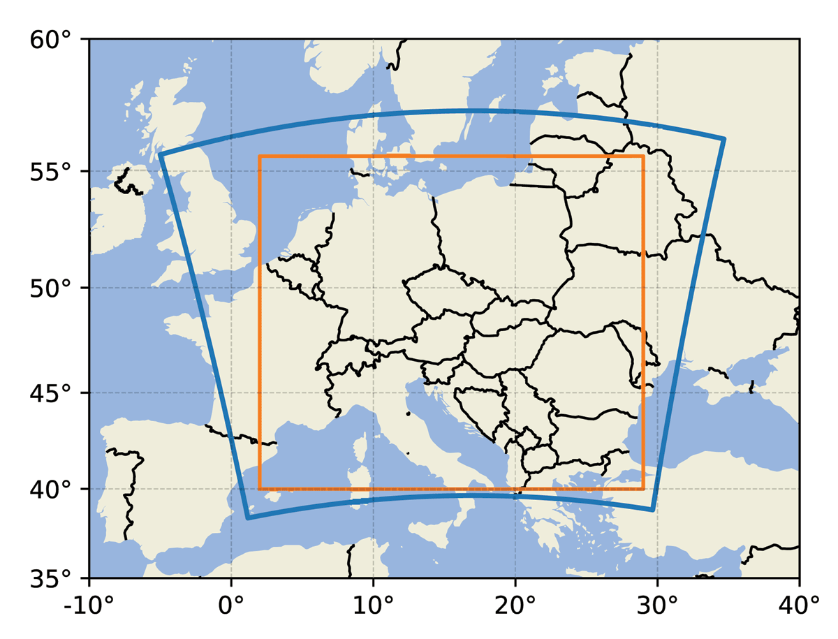
Figure 5
The model domain (blue quadrangle) and the verification domain (orange quadrangle).
For each period, an assimilation cycle is employed giving the initial state of model variables, including hydrometeors. The lateral boundary conditions are provided by the global model ARPEGE. They are updated every three hours with quadratic time interpolation in between. Hydrometeors are not coupled.
The moist deep convection scheme 3MT is active as the horizontal resolution of 2.325 km still lies in the gray zone of moist deep convection.
Three model configurations are tested:
EMP0 is the reference experiment using the two-ice scheme described in Section 2.
EMP1 with the three-ice scheme introduced in Subsection 3.1 with parameters for graupel parameterization listed in Table 1.
EMP2 with modifications introduced in Subsection 3.2 listed in Table 2.
The validation is divided into two parts. In the first part, the three-ice scheme represented by configuration EMP1 is compared to the configuration with the two-ice scheme EMP0. These two runs are compared for the period from 2022-02-16 to 2022-05-10 for runs starting at 00 UTC each day.
In the second part, the configuration EMP2 is compared to EMP1 for two periods. The first period is between 2022-06-20 and 2022-07-10, with frequent severe storms over Central Europe, especially in its first half. The second one is in autumn between 2022-11-08 and 2022-11-29, with enough precipitation but also with a short embedded stratocumulus period. For both periods, daily forecasts were initialized at 00 UTC.
4.2 Methods
4.2.1 Validation on standard atmospheric scores
The evaluation of experiments on the atmospheric scores is based on their comparison with SYNOP data and data from radiosondes. The southwestern and northeastern corners of the validation domain (Figure 5) are 40N, 2E and 55.6N, 29E, respectively. There are three statistics used:
where N is the number of measurements, Fi is the predicted value and Oi is the observed value of the evaluated quantity.
On top of that, the statistical significance of results is tested using a t-test with the null hypothesis such that the mean value of the differences in their statistics is equal to zero. Only significance levels of two and three multiples of the variance of the Gaussian distribution are considered, corresponding to roughly 95% and 99.73% confidence levels.
In addition, scores of radiation fluxes are verified against 19 Czech stations measuring shortwave radiation fluxes.
4.2.2 Fraction Skill Score
The Fraction Skill Score (FSS) is a method for the verification of precipitation following (Roberts and Lean 2008). Standard statistics like STDE and RMSE are prone to favor smoother precipitation fields over more variable ones with more misses and false alarms, although the less smooth ones might better capture the observed reality. This phenomenon is often called a double penalty, which origins from comparing data point by point without considering the spatial distribution of precipitation (Řezáčová et al. 2015). In contrast, FSS evaluates exceeding several precipitation accumulation thresholds in square boxes of specified areas, of which lengths of their sides usually increase in powers of two to overcome the above-mentioned deficiency. The asymptotic FSS shows the score of the biggest square with a side length of 301 km.
At CHMI, observational data are provided by the MERGE product (Novák and Kyznarová 2016), which combines the data from rain gauges from Czech stations with radar estimates of precipitation based on CAPPI 2 km; that is, from the closest radar beam to 2 km above mean sea level. The validation domain of FSS is Czechia, which is masked out to ensure good quality data obtained from the MERGE product (Bučánek 2020). If the cloud base is low and the precipitation phase is mixed, the MERGE composite might be biased because the precipitation rates are enhanced below that radar beam, and the rain gauges do not necessarily collect all snow due to wind. Therefore, some wariness is necessary while interpreting the results, especially in winter. Moreover, the data quality significantly drops outside of Czechia because there are no data from rain gauges.
Although the MERGE product delivers high-quality data for verification, some caution is needed when interpreting the data.
The main deficiency lies in the undercatchment by the gauges, especially of snow in windy situations. Another source of error is the recomputation of the radar reflectivities to estimates of precipitation accumulations and their adjustment based on the data from rain gauges.
4.2.3 Diagnostics in Horizontal Domains
Diagnostics in Horizontal Domains, abbreviated as DDH (Joly et al. 2019), is a valuable tool for assessing the impacts of tested modifications. It diagnoses the impact of various processes on the final tendency of a meteorological quantity at every model level. It offers diagnostic of many quantities, including temperature (enthalpy) and water species. Comparing several model runs of different configurations is possible. The domain of interest lies between (42.5N, 5E) and (55N, 25.5E) in the LCC map projection, a bit smaller than for standard atmospheric scores.
5 Results
5.1 Comparison of three-ice scheme to two-ice scheme
The model configuration EMP1 was compared to the EMP0 reference for the period from 2022-02-16 to 2022-05-10 in a so-called parallel suite.
Only minor differences are seen in the upper air scores (not shown). The surface scores (Figure 6) are also not changed significantly, but they reveal a reduction of STDE for temperature and relative humidity for some terms. The bias of temperature shows a general warming, except for 12 UTC. There are two causes: reduced evaporation of precipitation due to the higher fall speed of graupel and enhanced cloud cover by adjusted WBF coefficient. The latter dampens the diurnal cycle of temperature, causing daily maxima to be lower and minima higher. The differences are 0.02–0.03 K for maximum and 0.03–0.04 K for minimum temperatures each day of model forecast, so the difference is rather small. Contrary, the bias of geopotential reduced to the sea level is increased. Lower evaporation rates cause lower humidity at 2 meters, slightly improving its bias.
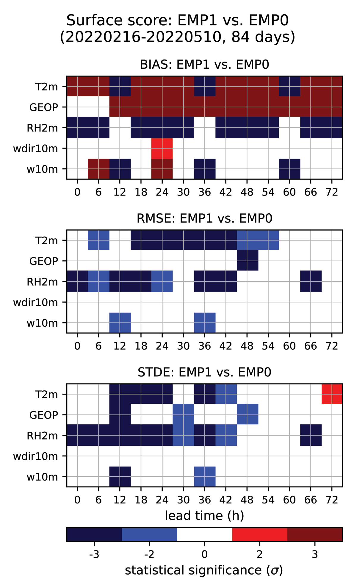
Figure 6
Statistical significance of the difference in bias, RMSE and STDE at the surface. Model configuration EMP1 is compared to EMP0 for the period from 2022-02-16 to 2022-05-10. Negative values of STDE and RMSE (in blue) mean improvement of EMP1 over EMP0, positive (in red) the opposite.
The asymptotic FSS (Figure 7) shows that the score is improved for precipitation accumulations thresholds 20 mm/6h and higher. Although the threshold of 20 mm/6h was exceeded only at one tenth of cases, the results should be credible as the total sample size is 960. However, Figure 8 shows that this phenomenon is mainly caused by overestimating higher precipitation accumulation. Some level of caution is needed when interpreting these data, because a significant part of the period was in winter, when undercatchment is expected.
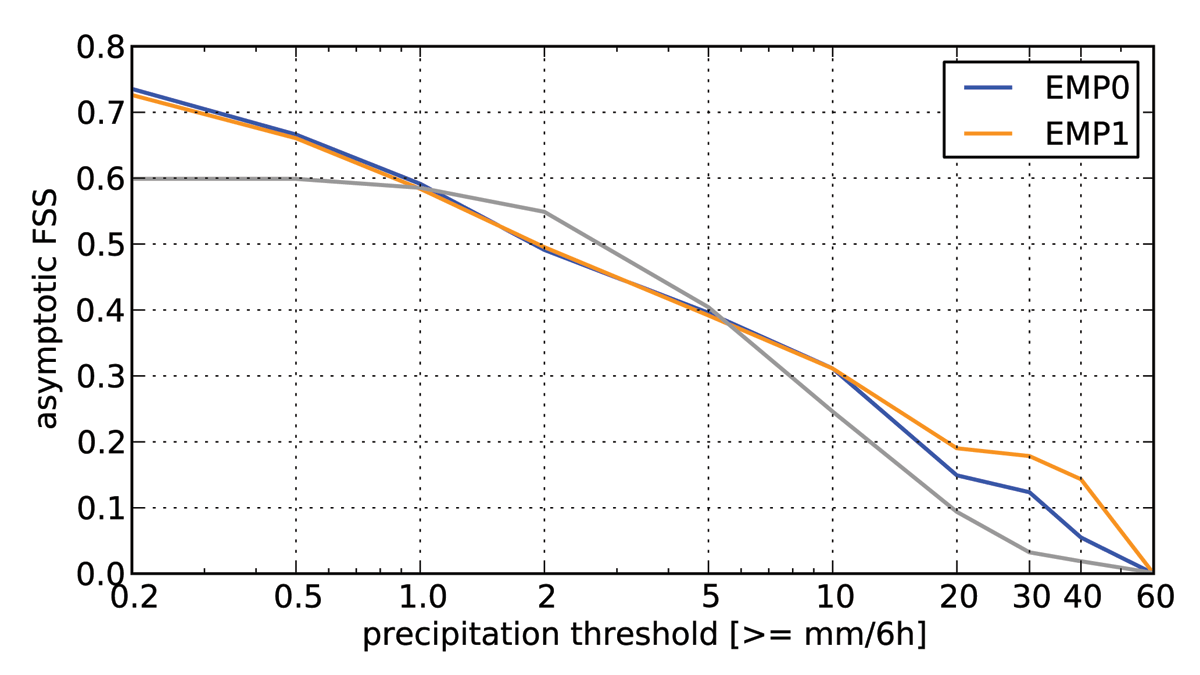
Figure 7
Asymptotic FSS for the period from 2022-02-16 to 2022-05-10, EMP0 in blue, EMP1 in orange. The mean of 6-hour precipitation accumulations over all runs and lead times is shown. In gray, the fraction of cases that exceeded the threshold is shown.
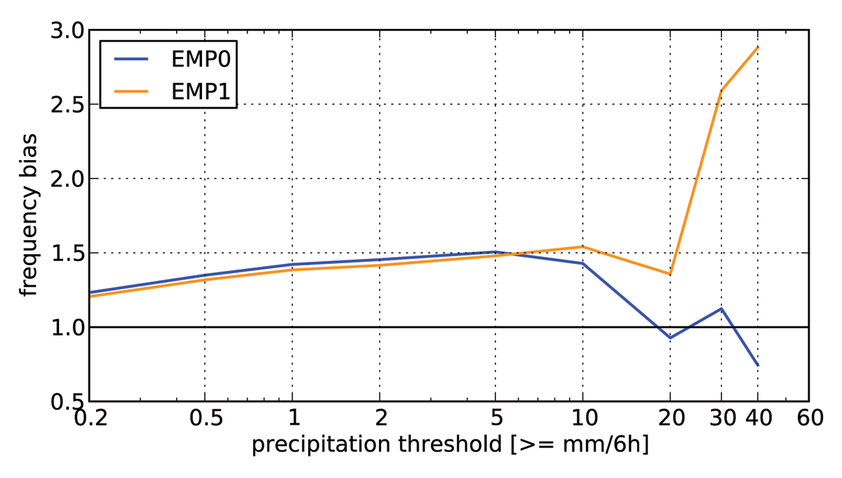
Figure 8
Precipitation frequency bias for the period from 2022-02-16 to 2022-05-10, EMP0 in blue, EMP1 in orange. The mean of 6-hour precipitation accumulations over all runs and lead times is shown.
The scores of global radiation for Czech stations (Figure 9) show a decrease in its positive bias. Its STDE is not significantly changed (not shown).
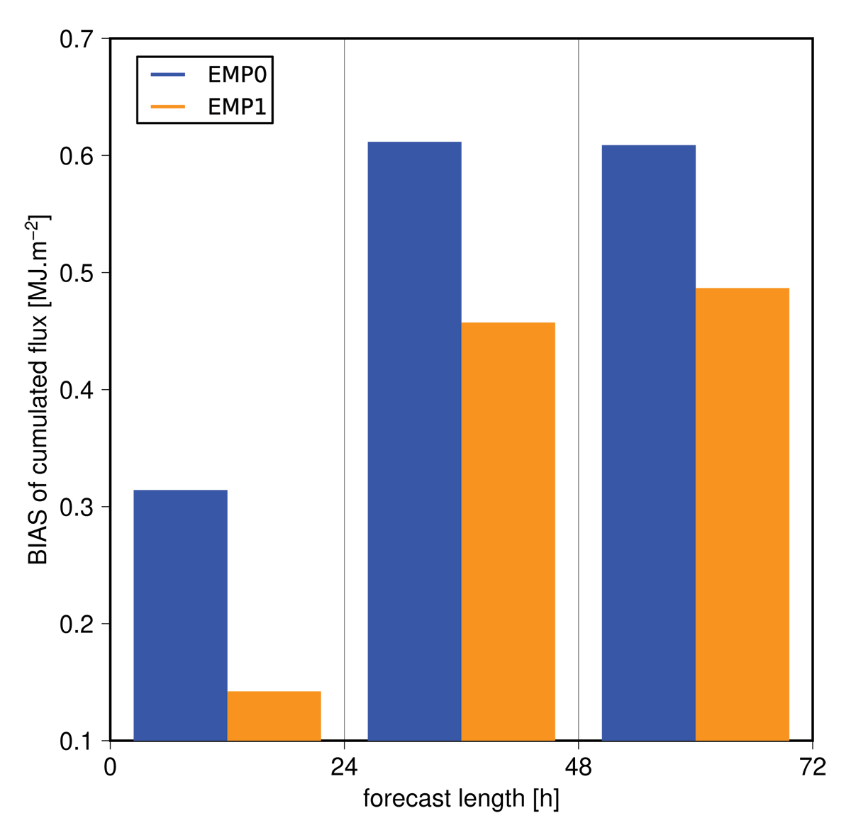
Figure 9
Comparison of global radiation for 19 Czech stations between EMP1 (orange) and EMP0 (blue) for the spring period between 2022-02-16 and 2022-05-10.
In addition to the validation over this longer period, selected summer, autumn, and winter cases were tested to assess the characteristics of the scheme in various weather regimes. Based on these tests, as well as on the long parallel suite, multiple key differences were revealed.
First, as expected, there is less snow as a perceptible fraction of ice hydrometeors is in the form of graupel. As a consequence, this lowers the simulated radar reflectivity of the upper parts of cumulonimbi. Figure 10 shows the maximum simulated reflectivity over the domain at every model level on 2022-06-24, averaged over all snapshots taken at the top of each hour. That day, a mesoscale convective system developed in the afternoon. While the reference configuration EMP0 has its maximum at higher levels around 5 km, where the solid phase predominates, EMP1 moves the maximum radar reflectivity to altitudes below 2000 m, where the precipitation is liquid. Reflectivities over 60 dBZ do not occur in model data as the scheme does not simulate hail.
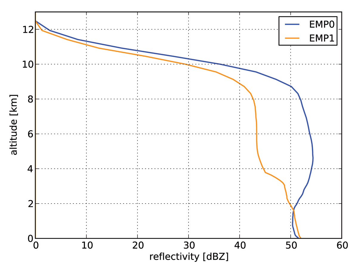
Figure 10
Average of all snapshots of maximum radar reflectivity at each model level at the top of every hour of the 24-hour forecast on 2022-06-24. Orange: EMP1, blue: EMP0.
Second, the vertical stratification of the troposphere is less stable (mainly in convective cases) due to less sublimation of graupel compared to snow. The left panel in Figure 11 shows the change in the temperature profile, and the right panel shows the contribution of evaporation to the water vapor budget.
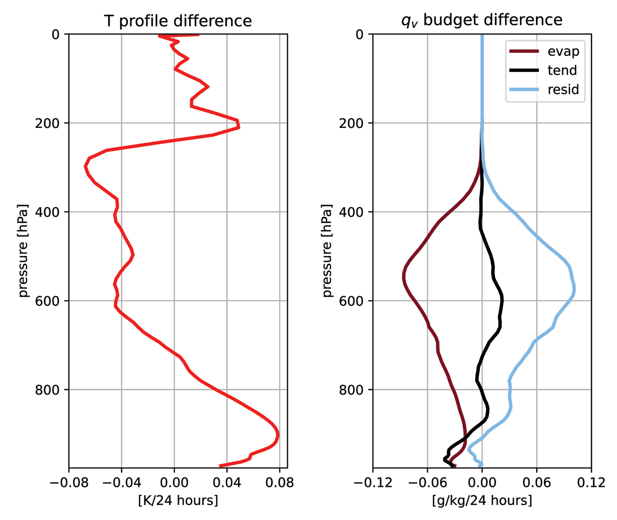
Figure 11
The 24-hour evolution of the difference in the vertical profiles of temperature (left panel) and qv (right panel) on 2022-06-24. Configuration with the 3-ice scheme is compared to the 2-ice scheme configuration. The contribution of evaporation is also plotted for qv.
Third, higher precipitation accumulations over mountains are simulated due to the faster fall speed of graupel, mainly in winter when the solid phase is in the whole vertical column. The higher fall speed reduces the precipitation spread, making the maxima higher with prognostic graupel than without it. This pattern is especially distinct if the shape of the mountain range is elongated and perpendicular to the prevailing winds, but it is also observed over the Alps and Carpathian Mountains. Figure 12 shows a 72-hour precipitation accumulation difference between EMP1 and EMP0 with a distinct increase in precipitation maxima over the Black Forest and Vosges mountain ranges.
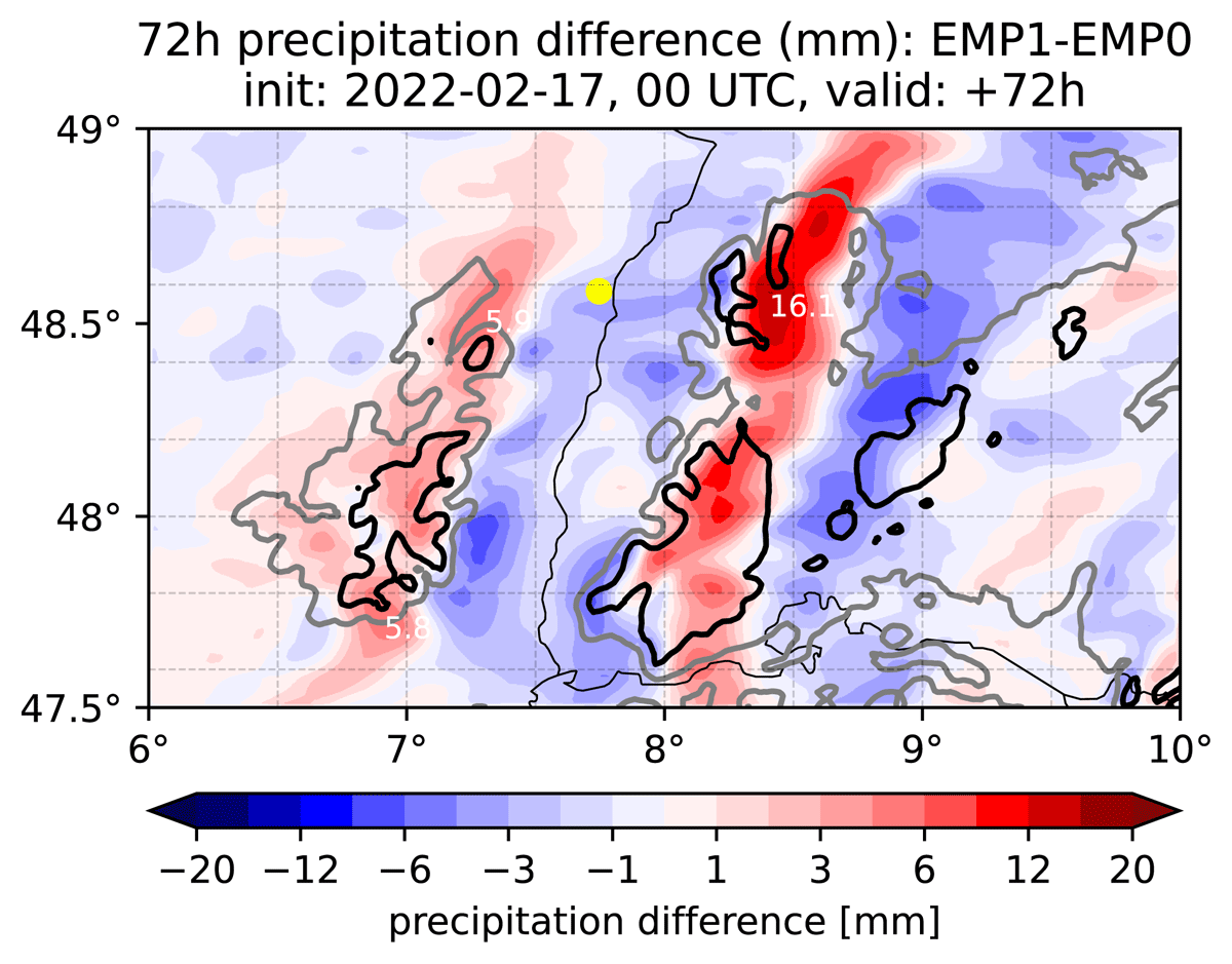
Figure 12
The difference in the 72-hour precipitation accumulations (EMP1-EMP0) starting on 2022-02-17 at 00 UTC. Note the increased precipitation maxima over the Black Forest and Vosges mountain ranges with a subtle reduction of precipitation in the Rhine valley near Strasbourg, marked by the yellow circle. The grey isoline shows the model surface altitude of 500 m, the black one of 800 m above sea level.
Finally, precipitation maxima in convective regions are higher with prognostic graupel. Although this effect differs from the increase in precipitation accumulations over mountains, it is again a consequence of the higher fall speed of graupel compared to snow. The destabilization of the troposphere, which is a consequence of the altered evaporation rates due to the faster fall speed of graupel, might also contribute to this effect. We experimentally assessed that the fall speed of graupel does not change the maximum precipitation accumulations much unless it is set to a very low value comparable to the fall speed of snow. There is also no significant sensitivity to values of autoconversion coefficients and collection efficiencies. Although the verification of precipitation maxima is challenging, it seems that they might be occasionally overestimated.
Due to reduced sublimation, which is a consequence of higher fall speeds, graupel can accumulate in higher amounts close to the melting layer, fall through it, and melt. The highest instantaneous precipitation fluxes in convective storms are usually located beneath such areas with high graupel content. It then causes higher instantaneous precipitation fluxes on the ground delivered by the three-ice scheme than the two-ice scheme. Although the instantaneous fluxes of the three-ice scheme are higher compared to the two-ice scheme, they are not unrealistically high with respect to observations. Hence, the reasons for high precipitation accumulations might possibly be too slow movement of storm cells or too broad an area of heavy precipitation rather than overshooted instantaneous precipitation maxima. However, the exact description of the mechanism of the occasional overestimation of precipitation accumulations with prognostic graupel remains unrevealed.
5.2 Validation of new microphysics options
5.2.1 Performance in summer
Firstly, configuration EMP2 is compared to reference EMP1 for a summer period between 2022-06-20 and 2022-07-10 with many convective storms over the model domain.
The modification of evaporation has a major effect on model results. The augmented evaporation rates impact the vertical stratification of the troposphere as higher evaporation rates consume more latent heat. If the reduction of evaporation of rain following Equation (4) is not used, the split of temperature contributions between dynamics and turbulence near the surface differs from the reference EMP1 (Figure 13). It is a consequence of the altered stratification of the lower troposphere. The difference in the accumulated turbulent flux of temperature (pointing downwards) over 24 hours (Figure 14) is negative near the surface. However, it abruptly turns positive, suggesting a compensating mechanism triggered by turbulence to reduce the increased stratification. Preliminary tests showed that the near-surface performance of wind speed and direction is consequently worsened. Employing the reduction of evaporation of rain solved the deterioration of wind scores. Thus, it is used in the final configuration EMP2, which is validated here.
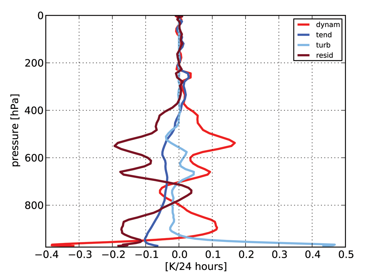
Figure 13
The temperature budget difference between a run with Lopez evaporation without reduction of evaporation and EMP1. Note the different split of contributions between turbulence (light blue) and dynamics (red), which was found to be responsible for worsening of the STDE of wind at 10 m. The selected case is on 2022-06-24.
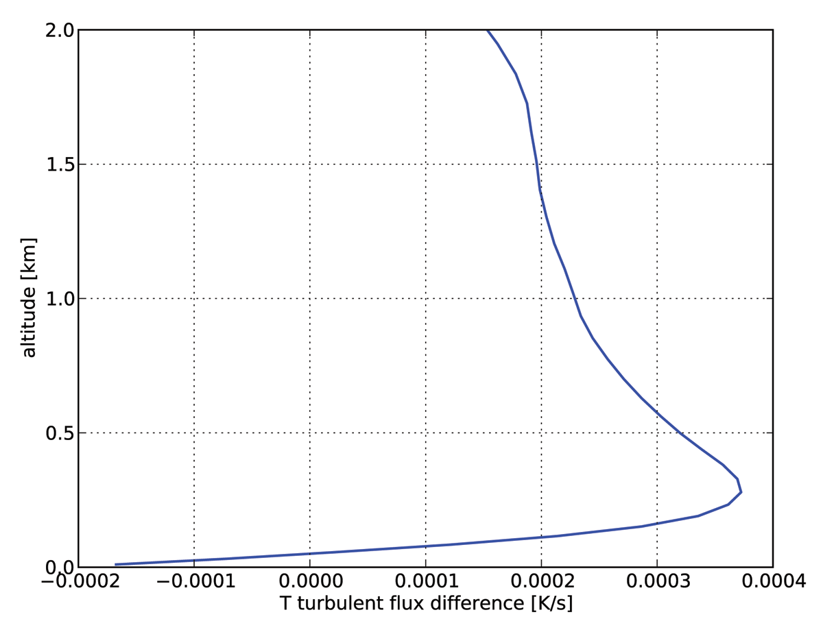
Figure 14
The difference in the accumulated turbulent flux of temperature over 24 hours. Configuration EMP2 is compared to the reference EMP1.
The upper air scores are very similar for both model configurations except for the bias of relative humidity, which is reduced due to the increase in relative humidity in EMP2. The surface scores are also comparable, except for a slightly reduced bias of the minimum daily temperature, which is reduced by approximately 0.05 K. This tendency is caused by a slightly reduced cloud cover, which enhances the outgoing long-wave radiation fluxes. The global radiation fluxes for Czech stations seem very similar for both configurations.
The asymptotic FSS (Figure 15) shows that EMP2 scores slightly better for the middle ranges of precipitation accumulations between 2 and 10 mm/6h but scores worse for heavy precipitation with thresholds of 20 mm/6h and higher. The threshold of 60 mm/6h was exceeded for almost 20% of 252 cases, which is a sufficient number of cases. The positioning of precipitation exceeding thresholds higher than 20 mm/6h is also worsened, except for the threshold of 60 mm/6 h, of which FSS of EMP2 is slightly better for square sides of 20–200 km lengths.
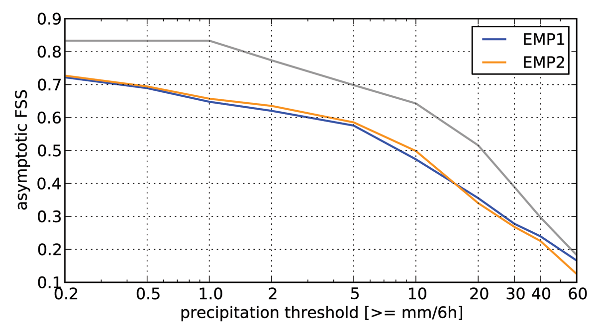
Figure 15
Asymptotic FSS for the 6-hour precipitation accumulations for EMP1 (blue) and EMP2 (orange) for the period from 2022-06-20 to 2022-07-10. In gray, the fraction of cases that exceeded the threshold is shown.
Figure 16 shows that the frequency bias of exceeding precipitation thresholds of 10 mm/6 h and higher is lower, although the difference is not huge. It also shows that EMP1 and EMP2 generally underestimate the lower precipitation thresholds but overestimate the higher ones, although the errors are not huge.
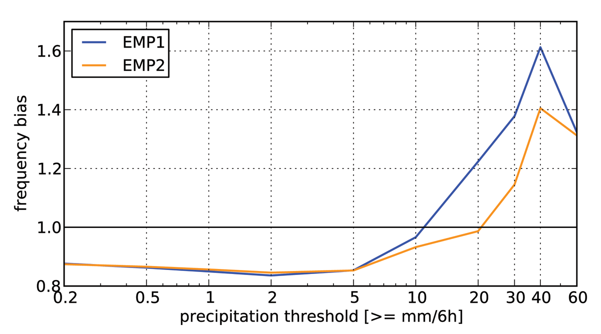
Figure 16
Precipitation frequency bias for the period from 2022-06-20 to 2022-07-10, EMP1 in blue, EMP2 in orange. The mean of 6-hour precipitation accumulations over all runs and lead times is shown.
The precipitation field can be significantly changed in convective storms. Especially, if the lower and middle troposphere in the vicinity of the storm is dry, the more effective evaporation of both solid and liquid precipitation contributes to the reduction of precipitation accumulations. One such case when a distinct reduction of precipitation accumulation in convection occurred was the night from 2022-06-28 to 2022-06-29 when a mesoscale convective system crossed Czechia. This convective storm weakened after crossing the hills in the south of Czechia. A significant reduction of precipitation accumulation over Northern Czechia is apparent in Figure 17. The key role of the changes in microphysics was verified by using initial conditions from EMP1 (not shown), which was tested to filter out the influence of the assimilation cycle.
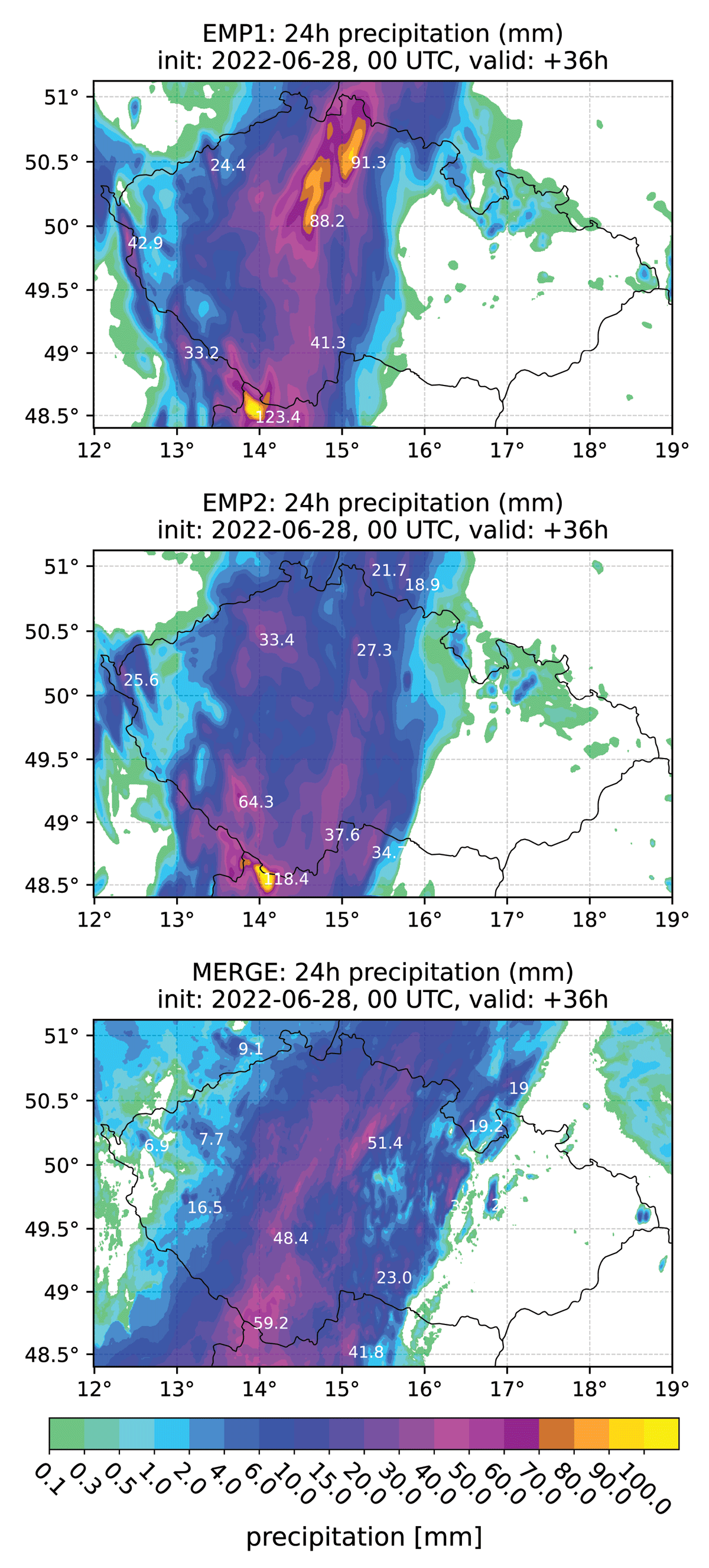
Figure 17
24-hour precipitation accumulations forecasted by EMP1 (top) and EMP2 (middle) ending at 12 UTC on 2022-06-29 compared to MERGE (bottom). Both model runs were initialized at 00 UTC on 2022-06-28.
5.2.2 Performance in late autumn
Secondly, the performance for the autumn period between 2022-11-08 and 2022-11-29 is evaluated. In this period, frequent fronts crossing the model domain occurred, as well as a five-day embedded period when stratocumulus prevailed over Czechia.
Version EMP2 reduces precipitation accumulations (Figure 18). Although the bias remains positive, undercatchment of precipitation in gauges is highly probable in this period.
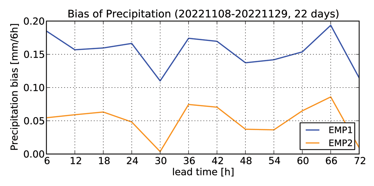
Figure 18
Six-hour precipitation accumulation bias for EMP1 (blue) and EMP2 (orange) for the period from 2022-11-08 to 2022-11-29.
The asymptotic fraction skill scores confirm the reduced precipitation bias (Figure 19). Configuration EMP2 scores higher for precipitation thresholds lower than 1 mm/6h. The principal source of these changes is the more effective Lopez evaporation parameterization, which reduces mainly lower precipitation accumulations when the cloud base is high enough to allow effective evaporation. In the case of drizzle, when the cloud base is low, or in the case of fog, the raised threshold of cloud water to rain autoconversion also reduces precipitation bias. The scores of precipitation accumulation thresholds between 1 and 5 mm/6h are comparable regarding the bias, but the location of precipitation is slightly improved (not shown). Asymptotic FSS is also improved for heavy precipitation exceeding 10 mm/6h. However, this threshold was exceeded only in less than 10% of 216 cases, which might not be a sufficient occurrence for making a trustworthy conclusion.
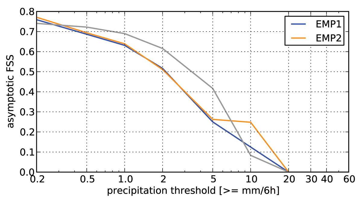
Figure 19
Asymptotic FSS for the 6h precipitation accumulations for EMP1 (blue) and EMP2 (orange) for the period from 2022-11-08 to 2022-11-25. The mean of 6-hour precipitation accumulations over all runs and lead times is shown. In gray is the fraction of cases when the given threshold was exceeded.
The upper air scores are generally neutral. The only improvement is an increase in relative humidity, compensating for its negative bias, similar to the summer period. The surface scores (Figure 20) occasionally show a warming trend, reducing the cold bias. The RMSE of 2-metre temperature is improved for all forecast times on various levels of statistical significance. The differences in the daily maximum and minimum temperature biases are lower than 0.02 K. Otherwise, the surface scores are rather neutral.
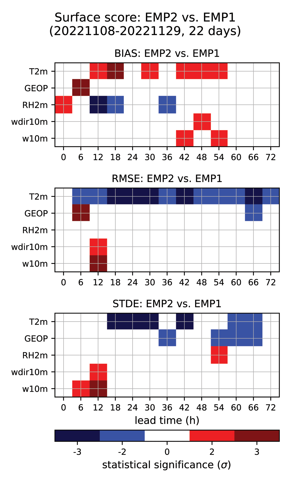
Figure 20
Statistical significance of the difference in bias, RMSE and STDE at the surface. Model configuration EMP2 is compared to EMP1 for the period from 2022-11-08 to 2022-11-29. Negative values of STDE and RMSE (in blue) mean improvement of EMP1 over EMP0, positive (in red) the opposite.
The cloud cover is augmented as a consequence of raised evaporation rates, slightly reducing the positive bias of global radiation for Czech stations. Figure 21 shows that the bias of global radiation still remains positive for this period, pointing out a persisting lack of cloud cover. Its STDE is rather neutral or subtly reduced.
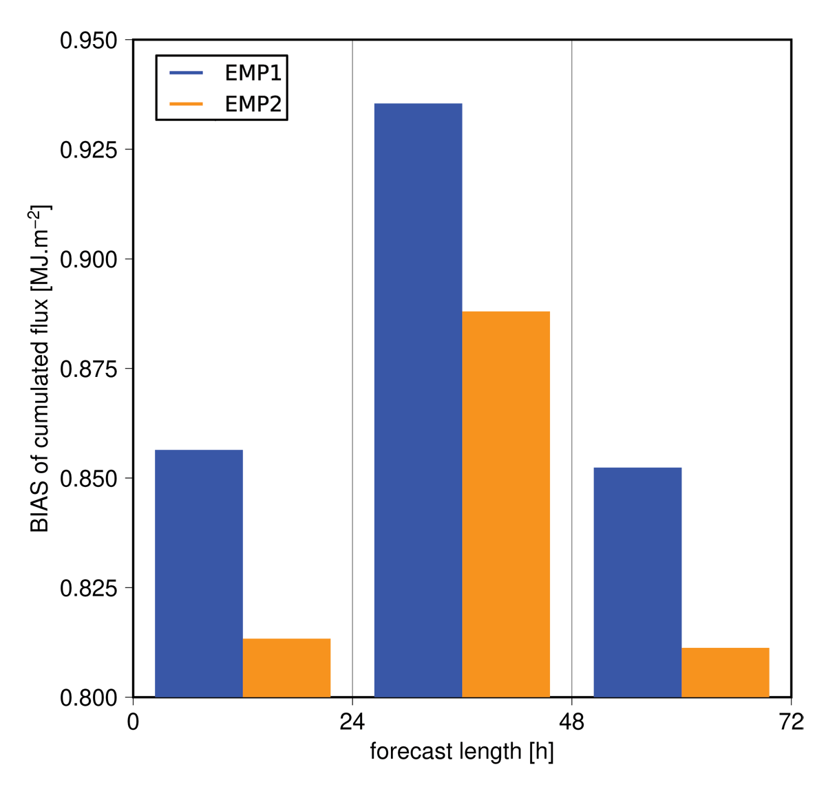
Figure 21
Comparison of global radiation fluxes for 19 Czech stations between EMP2 (orange) and EMP1 (blue) for the autumn period between 2022-11-08 and 2022-11-29.
The precipitation shadow behind mountains is more pronounced with the new evaporation parameterization. One such case is shown in Figure 22 with a more distinct precipitation shadow behind the Ore Mountains. The precipitation phase was mixed, where most precipitation was liquid in the lowlands, and both phases contributed approximately equally to the precipitation accumulation over the Ore Mountains. Due to that, some undercatchment of precipitation by rain gauges is expected, as well as weaker radar echoes, as precipitation might be enhanced due to collection below the radar beam at 2 km.
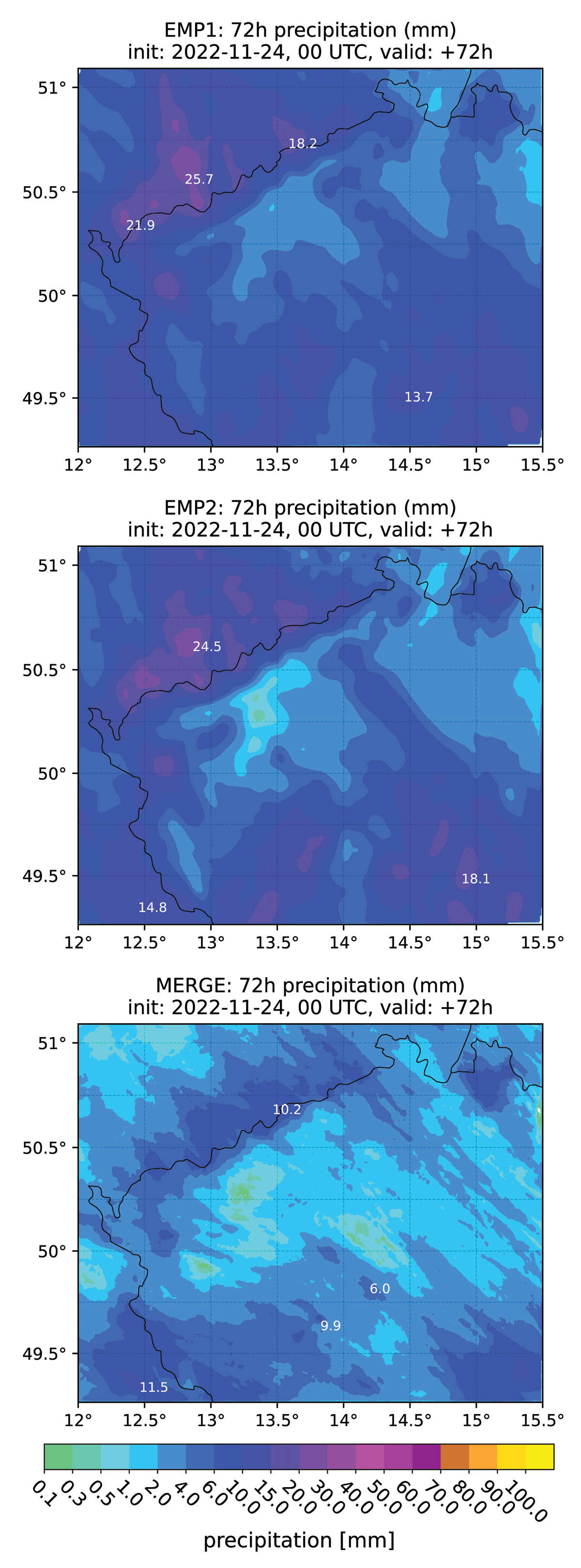
Figure 22
72-hour precipitation accumulations forecasted by EMP1 (top) and EMP2 (middle) ending at 00 UTC on 2022-11-27 compared to observations by MERGE (bottom). A precipitation shadow is distinct diagonally on the Czech side of the German-Czech border, which lies on the top of the main ridge of the Ore Mountains, as precipitation moved from northwest to southeast. Although rain, snow, and graupel contributed to the precipitation accumulation, rain was dominant except for the highest parts of the mountains, where the amounts of solid and liquid precipitation accumulations were equal.
6 Discussion and Conclusion
In this article, graupel was introduced as a prognostic variable in the microphysics scheme in ALARO and further microphysics developments of this scheme were presented.
Graupel is produced by the WBF process, freezing of rain, it collects cloud ice and cloud water and its sink terms are sublimation, melting, and sedimentation. The WBF process, as well as the freezing of rain, produce graupel in the three-ice scheme, unlike in the two-ice scheme, in which they produce snow. Graupel particles are assumed spherical with a constant density of 400 kg∙m–3. Their size distribution is described by the Marshall-Palmer distribution with the intercept parameter N0,g = 4∙106 m–4. The terminal fall speed of graupel is lower compared to rain but higher than snow. This set of parameters introduces a faster-falling ice particle to the scheme. Despite the parameterization of graupel having many uncertainties, the choices of parameters intend to represent an average value of graupel properties.
This proposal for graupel parameterization was compared to the two-ice scheme model configuration for an almost three-month period in spring 2022. The results show a small improvement in the upper air scores of temperature below 500 hPa, where the bias is reduced, as well as its STDE. In addition, several key dissimilarities between the two-ice and three-ice schemes were revealed in additional selected cases:
Less snow reduces radar reflectivities in the upper parts of convective storms.
The troposphere is less stable due to less sublimation of graupel compared to snow, mainly in summer. This causes the warming of the lower troposphere.
Precipitation maxima over mountains and in convective storms are higher. This might be caused by the higher fall speed of graupel compared to snow, which is often observed in localized high amounts near the melting layer. The destabilized troposphere, which is a consequence of less evaporation due to faster-falling graupel, might also contribute to this effect.
The introduction of prognostic graupel influences the precipitation structure and bias of higher precipitation accumulations. However, the total precipitation bias is not much altered as it seems to be more sensitive to modifications of parameters of microphysics processes.
The rates of microphysical processes were adjusted in addition to the modifications of the parameterization of graupel. A set of further microphysical developments for all precipitating hydrometeors was presented:
The coefficients of autoconversion to rain and snow and threshold values of autoconversion to rain were modified, while the new computation of cloud ice to snow autoconversion threshold was not retained. This combination of adjustments helps to maintain good geopotential scores with little impact on the precipitation field.
The Lopez evaporation scheme was extended for use in ALARO with prognostic graupel, replacing the previously used Kessler scheme.
Parameters of the yearly cycle of the decorrelation length for the exponential-maximum-random overlap and the vertical profile of critical relative humidity in the cloud scheme in radiation were adjusted to maintain good model results, which were mainly affected by the Lopez evaporation scheme.
This set of microphysics developments was validated for 72-hour model integrations on 22 consecutive days in two periods, one in summer 2022 and the other in November 2022. The main benefit of this microphysics package is a reduction of the positive bias of precipitation accumulation in the autumn period. The enhanced evaporation rates occasionally reduce the overestimated precipitation maxima in convective storms, although they still often remain overestimated. The reduction is not observed in all cases due to many feedbacks in convection. Finally, the precipitation shadow behind mountains is more distinct, improving its simulation.
Evaporation is the decisive process for reducing precipitation bias only when the cloud base is high above the ground. When the cloud base is close to the ground or in the case of fog, the lack of time for possible evaporation prevents it from affecting precipitation. In such cases, autoconversion is the paramount process impacting the precipitation field. The two opposite autoconversion modifications, which are the increased threshold value of cloud water for the autoconversion to rain and the raised autoconversion coefficient for rain, roughly equalize their influence on the precipitation field in the case of drizzling stratus.
The final proposal proves its skill in NWP and is also expected to improve climate simulations.
Appendices
Appendix A: Parameterization of microphysical processes
A1 Autoconversion
The Sundqvist type of autoconversion (Sundqvist 1978) is used for the autoconversion to rain and snow, written as (Catry 2006)
where kr/s are the autoconversion coefficients for rain and snow and are the threshold values of ql/i above which autoconversion occurs if the Heaviside step function is used instead of this smoother transition function.
Unlike , the value of is temperature dependent, written as
with and constants. The coefficient ks is also temperature dependent as
where ks,0 is a constant, T is temperature, and Tt is the temperature of the triple point of water. The constant in the exponent was obtained by averaging multiple temperature dependencies proposed in Lopez (2002).
The Wegener-Bergeron-Findeisen (WBF) process contributes to the growth of the snow category in the two-ice scheme or it produces graupel in the three-ice scheme. The WBF process is treated as a special case of autoconversion (Geleyn et al. 2007):
where are tuning parameters with recommended values of and (Geleyn et al. 2007).
A2 Collection
The continuous growth model is used for the description of collection in ALARO. Here, we describe the collection of cloud water by rain with the Marshall-Palmer size distribution. Other collection processes are parameterized in the same way. One begins from (Catry 2006):
where Er is the collection efficiency of rain, D the diameter of a raindrop, and a with α are parameters for fall speed of a drop wr.
Equation (A5) leads to the final equation:
where Ccol = 0.335 in SI units and Rr is the precipitation flux of rain.
A3 Evaporation
The equation for the Kessler evaporation parameterization describing the loss of mass fraction of rain due to evaporation or sublimation is written as (Catry 2006)
where b(T,p) is a function dependent on temperature T and pressure p, β is a parameter, mr is the mass of rain, and qw is the saturated value of qv over liquid water at the exact temperature of saturation when the latent heat release is considered. Equation (A7) leads, after comparison with the data from Smithsonian meteorological tables, to the final expression in the flux form:
A4 Melting
Melting is parameterized similarly to evaporation, when only the ratio of the specific heat of melting to the heat capacity of water must be considered modifying Equation (A7) to (Catry 2006):
for T > Tt with b′ = bB (the same b as in Appendix A3), B = γcpd/dvLf, where γ is the thermal diffusivity of air, cpd the specific heat capacity of dry air at the standard atmospheric pressure, dv the molecular diffusivity of water vapor, and Lf the specific latent heat of fusion.
The final equation in the flux form derived from Equation (A9) yields
where xs is the snow fraction of the precipitation flux and Rs is the snow precipitation flux.
A5 Abel-Boutle size distribution
For rain, ALARO uses a negative exponential size distribution with the intercept parameter recommended by Abel and Boutle (2012), written for the number concentration of droplets N as a function of the drop diameter D as:
where x1 = 0.22, x2 = 2.2, and
A6 Partition between cloud water and cloud ice
The partition of condensates between cloud water and cloud ice if T < Tt follows equation:
where cpart is a tunable parameter and Tx is the temperature of the highest difference between saturation water vapor pressure over liquid water and ice.
Acknowledgements
The authors would like to thank Bogdan Bochenek from the Institute of Meteorology and Water Management, Poland for his work on the inclusion of prognostic graupel into the ALARO code. The authors would also like to thank Petr Novák from the Czech Hydrometeorological Institute for providing precipitation estimations MERGE. The authors would like to thank two anonymous referees for their helpful suggestions.
Funding Information
David Němec and Radmila Brožková would like to thank the Technology Agency of the Czech Republic for its financial support under the grant no. SS02030040 (Prediction, Evaluation and Research for Understanding National sensitivity and impacts of drought and climate change for Czechia, PERUN).
Competing Interests
The authors have no competing interests to declare.