
Introduction
As the environmental impacts of burning fossil fuels to produce energy become strongly prominent, coupled with energy security issues triggered by recent conflicts in Eastern Europe, the search for efficient and environmentally friendly energy sources becomes increasingly important. Out of all renewable energies, solar power remains one of the most prominent. According to the International Energy Agency (IEA, 2022), an upward revision of renewable energy growth for the next five years has been driven mainly by China, the United States and India, which are implementing policies and introducing regulatory and market reforms faster than previously planned to combat the energy crisis. Following this same trend, Brazil has increased its share of renewable sources in its energy matrix, notably solar photovoltaics one. With strong growth of more than 86% per year in its installed capacity in the last five years, photovoltaic energy is the source that has grown the most, constituting today the second largest source of electrical energy, accounting for more than 15% of the Brazilian electrical matrix, about 70% as distributed energy systems (ANEEL, 2023; ABSOLAR, 2023). The country has advantageous conditions for the implementation of solar photovoltaic sources, especially the Northeast region (i.e., Paraíba, Bahia, Pernambuco, amongst others), North of Minas Gerais, and São Paulo, as well as the Central-West with mean annual of daily total solar irradiation rates on the inclined plane in the range of 5.50–6.25 kWh.m-2.day–1 and low seasonal variability due to their situation geographically mostly in the Inter-tropics (Pereira et al., 2017). This increase in solar energy is a major step forward in the trend towards a clean energy transition in response to growing national energy consumption, which is now the object of greater attention. Since the solar photovoltaics source is primarily dependent on atmospheric conditions, theoretical simulation, and feasibility studies of solar energy generation projects, as well as architectural studies focused on energy efficiency and thermal comfort of buildings, must take this natural dependence into account. The impacts of the natural variability of meteorological conditions on photovoltaic energy production over the years is often analyzed using the Typical Meteorological Year (TMY) methodology (Hall, et al., 1978). A TMY dataset is widely used when modeling renewable energy systems to represent a long time period of data as a typical year. A TMY consists of 12 “Typical Meteorological Months” (TMMs), each of which is deemed the most typical compared to the long-term average for that calendar month (Skeiker, K., 2004; Skeiker, K., 2009; Chan, et al., 2006; Huld, et al., 2018). The generation of a TMY is preferable to simply using the average hourly data from a long time series, because a TMY consists of 12 months of real data. The long-term average time series would consist of synthetic data that did not actually occur, meaning that some element of the natural variability of the weather at that location is lost. However, TMYs represent typical and not extreme conditions for a given location. Evaluating extreme cases requires other methodologies.
Although TMY data are available for Brazil from other sources (e.g., Luiz et al., 2012; Almeida & Vasconsellos, 2019; Machado et al., 2019; Bonini, et al., 2022), detailed studies on the sensitivity of the results in relation to the data source and weighting factors are not available. In this article we tested three different data sources: in-situ observational data, satellite model data and reanalysis data, which gives this work its originality.
In this study a TMY dataset was generated for the five distinct climatologically regions in Brazil shown in Figure 1 using a variation of the method proposed by Hall et al., 1978. This method applies Finkelstein-Schafer, 1971 (named as FS) statistics to a long time series of data to determine months which are most “typical” compared to the long-term average, and then concatenates these months into a TMY. The typical months are selected on the basis of 10 daily meteorological indices consisting of the maximum, minimum and average values of air temperature and relative humidity, maximum and average wind speed, global horizontal solar irradiation and normal direct irradiation.
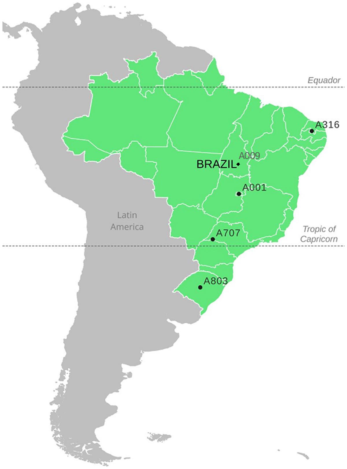
Figure 1
The five locations where the TMY’s were generated.
Since the TMY generation procedure proposed by the Sandia method (Hall, et al., 1978), and the notion of ‘typicality’ are somewhat subjective, in this paper we investigate the sensitivity of the resultant TMY to changes in the source of the data series, and to the weighting factors of the meteorological parameters. We obtain data from three different sources – ground observations, a satellite-derived model (Pereira et al, 2017), and atmospheric reanalysis from ERA5/ECMWF – for a 13-year period from 2005–2017. The TMY for each region is generated using 3 different data schemes to determine the sensitivity of the TMY to the data source. Moreover, we investigate the effect of changing the weightings of the daily weather indices when generating the TMY.
Methodology
The basis of the TMY generation procedure of this study is the application of Finkelstein-Schafer statistics (FS) to the hourly weather data of a 13-year period, allowing the selection of representative typical meteorological months (TMM’s). The choice of this statistical method was based on the results presented by the authors, which, according to them, proved to be more powerful than the Kolmogorov-Smirnov test for this type of application. The cumulative distribution function (CDF) for each individual year is compared to the long-term composite of the entire period for each of the selected daily weather indices, and the year with the closest CDF to the long-term composite is selected as the TMM. This is done for each calendar month, and the resultant 12 TMMs are concatenated to produce the TMY dataset.
Generation of Cumulative Distribution Functions (CDFs)
The TMY generation procedure begins from hourly data of the 13-year time period for the following meteorological parameters: air temperature, relative humidity, wind speed and solar radiation. Ten daily weather indices are generated from this hourly data: maximum, minimum and mean dry air bulb temperature (Tmax, Tmin, Tmean) and relative humidity (RHmax, RHmin, RHmean), maximum and mean windspeed (Wmax, W), daily global solar radiation (GHI), and direct normal solar irradiation (DNI). For each calendar month, each of the 10 sets of daily indices were sorted into bins, and the CDFs were calculated by counting the cases in each bin. For N observations of a variable x that are sorted into an increasing order x1, x2, …, xN, the CDF is given by the following function:
For each calendar month, a long term CDF is generated for the entire time period, as well as individual short term CDFs for each individual year. For example, for January, we calculate one long-term CDF consisting of the data for all 13 Januarys, as well as 13 individual CDFs for the January data from each year. This is done for each calendar month, and each daily index.
Using Finkelstein-Schafer statistics (FS), the monthly CDFs are compared to the long-term CDF for each index. This statistic gives a measure of the average absolute difference between the long-term CDF and the monthly CDF. The FS statistic for each index is calculated using the following equation (1):
where CDFm is the long-term CDF for month m and CDFy,m is the short-term CDF for month m in year y. N is the number of bins and x is the daily index.
The FS statistic is calculated for each calendar month, and for each daily meteorological index. To obtain a singular value for each calendar month, we must combine the FS statistics of every daily index. This can be done simply by calculating the sum of the FS statistics; however, this would assume that each daily index is equally as important as the others when determining the closeness of a month to its long-term average. For example, to generate a TMY for solar system performance, the global radiation is deemed to be much more important than the wind speed. In order to account for these differences, a weighted sum of the FS statistics is calculated, with different weighting factors corresponding to the importance of the daily index. In this study, we focus on TMY generation for solar energy systems, hence the significant weighting on radiation. A weighted sum of the FS statistics for the M daily indices is calculated using the following equation (2):
where the weighting factor, WFx, for each daily index can be found in Table, and the weighting factor, WFx, for each daily index is shown in Table 1.
Table 1
Weighting factors scheme used for calculating TMY and TMY3.
| SCHEME | Tmax | Tmin | RHmax | RHmin | Wmax | GHI | DNI | |||
|---|---|---|---|---|---|---|---|---|---|---|
| TMY | 1/24 | 1/24 | 2/24 | 1/24 | 1/24 | 2/24 | 2/24 | 2/24 | 12/24 | – |
| TMY3 | 1/20 | 1/20 | 2/20 | 1/20 | 1/20 | 2/20 | 1/20 | 1/20 | 5/20 | 5/20 |
This is the original weighting scheme suggested by Hall et al., 1978, however a modification was later suggested by Wilcox-Marion, 2008, to include Direct Normal Irradiance (DNI), rather than solely Global Horizontal Irradiance (GHI) and reduce the weighting on wind. Additionally, this later update to the Hall’s method utilized modelled solar radiation data. We refer to this updated Hall method as “TMY3”, and the weighting scheme for this method can be found in Table 1.
Later in this study, we investigate the use of different weighting schemes and investigate the sensitivity of the generated TMY to these weighting factors for weather indices. Various methods have been proposed in the literature (e.g., Marion-Urban,1995; Huang et al., 2014; Su et al., 2009), to select the final TMM once the weighted sums (WS) have been calculated. These involve imposing persistence criteria or calculating the root mean squared difference (RMSD), yet for the sake of simplicity for this paper we simply select the month with the smallest WS as our TMM.
The hourly data for each of the 12 TMMs are concatenated and smoothed for 6 hours on either side of month interfaces to account for discontinuities, thus producing the TMY. A final comparison of the CDF for the entire time period and the CDF of the TMY is calculated to demonstrate the closeness of the two datasets.
Data Used
The aims of this study were not only to produce a TMY for each of the 5 selected regions of Brazil, but also to compare the TMYs generated from different data sources. In theory, the TMYs generated from different sources of data should be the same for a specific location, however this study investigates whether we can be confident in the consistency of the TMY across different data sources.
The study used measured data from 5 stations collecting solarimetric data from the SONDA network (http://sonda.ccst.inpe.br/), representing the predominant climatic macro-regions in the country. The SONDA solarimetric network is maintained and operated by the National Institute for Space Research (INPE) and is linked to the Baseline Surface Radiation Network (BSRN-GEWEX), providing long-term and high-quality data series of solar irradiation, wind speed and other meteorological data. The stations were selected based on the representativeness of the climate, quality and continuity of the data and they are named: A009 Palmas – North A316, Caicó – Northeast; A001 Brasilia – Central-West; A707 Presidente Prudente – Southeast, and A803 Santa Maria – South.
It is difficult to obtain continuous hourly data for long time series of data (>10 years), so there are some gaps in the meteorological data provided. For short gaps in the data (less than 6 hours), the missing values are filled using linear interpolation based on previous values at that hour. For longer gaps, months containing more than 5 days of missing data (100 hours) were discarded from calculation of the TMY. This was done because otherwise a potential candidate for the TMM would contain more than 5 days of interpolated data, resulting in too much synthetic data in the TMY and defeating the purpose of using a TMY instead of the long-term average. In addition, a data quality control procedure was carried out to eliminate spurious values, such as non-zero solar radiation values at night or consistently unrealistic values for the chosen locations.
In TMY calculations, it is preferable to have as long a time period of data as possible to ensure that the long-term average is truly representative of the meteorological conditions in that region. In this study, we set our threshold for the sample size of years from which the TMM can be selected as 10 years. This enabled at most 3 months for each calendar month to be discarded. In some cases, we relax this condition to 9 years since it is difficult to obtain 10 years of reliable data in some areas of Brazil. For stations that did not meet this condition, an alternative station in that same region of Brazil was used to generate the TMY.
Ground observation data was obtained from automatic weather stations (AWS) from the Brazilian National Weather Service (INMET) located at the 5 locations of interest, as seen in Figure 1. For our initial TMY generation, hourly data for all 9 daily indices from these AWS stations was used. Since these stations do not contain data for Direct Normal Solar Radiation, the TMY weighting scheme from Table 1 was used to generate the observational TMY. The TMYs calculated from ground observation data are referred to as TMYobs throughout the remainder of this report.
Satellite and ERA5 Modelled Solar Radiation
Numerical assessment of downward incoming solar irradiance employed a satellite-derived model for the 5 locations of interest as shown in Figure 1. The numerical physical-based model Brasil-SR (Pereira et al, 2017)) estimated the solar radiation incident components on the surface (GHI and DNI), combining the use of the two-flux method in the solution of the radiative transfer equation with the use of parameters determined from satellite images. The radiative transfer calculations follow a two-stream approximation with δ-Eddington scaling to estimate the downward surface GHI and to derive the other solar radiation components (Pereira et al., 2017; CasaGrande et al., 2021). This time-series Irradiance Model uses more than 17 years of satellite data from GOES/NOAA to derive modelled Global Horizontal Irradiance (GHI) and Direct Normal Irradiance (DNI). The Brazil-SR model was validated based on more than 300 in situ measurements AWS data from INMET and other sources, and Table 2 shows the validation metrics of the monthly averages of daily total horizontal global irradiation for each one of the Brazilian regions.
Table 2
Benchmark of the Brazil-SR model.
| REGION | R | RELATIVE BIAS | RRMSE1 |
|---|---|---|---|
| North | 0.81 | 0.60% | 9.7% |
| Northeast | 0.87 | 0.20% | 8.3% |
| Central-West | 0.86 | 0.50% | 8.3% |
| Southeast | 0.91 | 0.10% | 8.4% |
This modelled radiation data was used to replace the Global Horizontal Radiation (GHI) data from the solarimetric station data and allows for a further two TMYs to be calculated for each location. The first of these, TMYmod, used only the modelled GHI data and therefore used the TMY weighting scheme. The second of these, TMY3mod, used both the modelled GHI and DNI data, thereby using the TMY3 weighting scheme.
The final source of data used in this project was the ERA5-Land Hourly Reanalysis data from ECMWF (Muñoz Sabater, 2019). Reanalysis data combines modelled data with observations to create a complete and consistent dataset. However, since reanalysis data often has difficulties in resolving clouds, in this study we use the modelled GHI and DNI data in combination with the ERA5 data for the other daily weather indices (temperature, wind velocity and relative humidity). We include both GHI and DNI, and therefore use the TMY3 weighting scheme. The TMY generated from this data is referred to as TMY3rea.
Results
Central-West: Brasilia/DF (A001)
For the Brasilia station, there were at least 10 years from which TMM could be selected for each calendar month, therefore no alternative station was needed. The TMY was generated for each of the four different data sources and can be found in Table 3.
Table 3
The generated TMYs for different data sources, with the final FS statistic values for the TMY CDF compared to the long-term average CDF.
| MONTH | YEAR | |||
|---|---|---|---|---|
| TMYOBS | TMYMOD | TMY3MOD | TMY3REA | |
| January | 2009 | 2009 | 2009 | 2009 |
| February | 2011 | 2012 | 2011 | 2012 |
| March | 2013 | 2013 | 2013 | 2009 |
| April | 2008 | 2007 | 2007 | 2017 |
| May | 2017 | 2014 | 2014 | 2006 |
| June | 2011 | 2015 | 2015 | 2017 |
| July | 2013 | 2012 | 2012 | 2007 |
| August | 2015 | 2013 | 2013 | 2013 |
| September | 2014 | 2014 | 2012 | 2012 |
| October | 2016 | 2016 | 2016 | 2016 |
| November | 2014 | 2017 | 2017 | 2016 |
| December | 2017 | 2010 | 2010 | 2006 |
| FS | 0.0065 | 0.0073 | 0.0094 | 0.0066 |
From the generated TMYs, we can see that there is agreement of at least 2 of the data sources for every calendar month, with 2 months (January and October) having the complete agreement of the TMM. The greatest similarity is between the TMYmod and TMY3mod results, with only 2 calendar months disagreeing, however this is not surprising since these TMYs only differ due to the inclusion of DNI in TMY3.
The CDF for each generated TMY is compared to the long term (LT) observed and modelled CDFs for the annual GHI, as shown in Figure 2. Evidently, these CDFs are extremely close to each other. The lower the value calculated for the Finkelstein-Schafer parameter, the closer the values of the two curves will be. In general, the calculated FS values are relatively low and close to each other, with the lowest value tabulated in Table 3 occurring for the observational data.
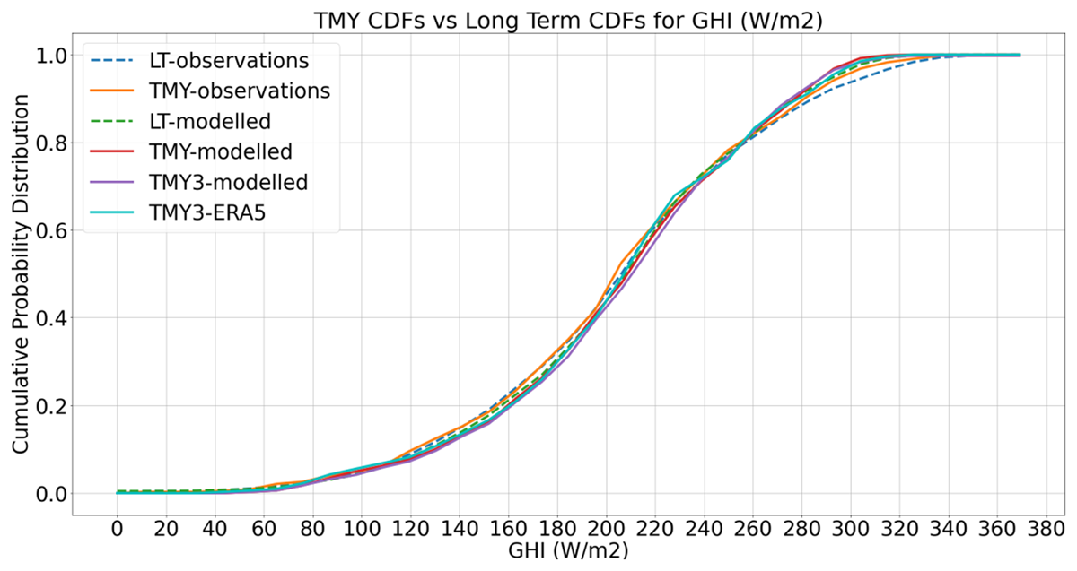
Figure 2
Comparison of the long-term average CDF and TMY CDFs for observed and modelled GHI.
Southeast: Presidente Prudente/SP (A707)
For the Presidente Prudente station, there were at least 10 years from which TMM could be selected for each calendar month, therefore no alternative station was needed. The TMY was generated for each of the four different data sources and can be found in Table 4.
Table 4
The generated TMYs for different data sources, with the final FS statistic values for the TMY CDF compared to the long-term average CDF.
| MONTH | YEAR | |||
|---|---|---|---|---|
| TMYOBS | TMYMOD | TMY3MOD | TMY3REA | |
| January | 2013 | 2009 | 2011 | 2016 |
| February | 2010 | 2008 | 2008 | 2016 |
| March | 2010 | 2017 | 2014 | 2009 |
| April | 2011 | 2010 | 2010 | 2017 |
| May | 2010 | 2013 | 2012 | 2013 |
| June | 2017 | 2015 | 2015 | 2015 |
| July | 2011 | 2011 | 2011 | 2005 |
| August | 2011 | 2013 | 2013 | 2013 |
| September | 2013 | 2013 | 2013 | 2013 |
| October | 2008 | 2011 | 2016 | 2011 |
| November | 2012 | 2012 | 2012 | 2017 |
| December | 2006 | 2005 | 2012 | 2012 |
| FS | 0.0134 | 0.0074 | 0.0062 | 0.0090 |
From the generated TMYs, we can see that there is agreement of at least 2 of the data sources for 10 calendar months, with 1 month (September) having the complete agreement of the TMM.
The CDF for each generated TMY is compared to the long term (LT) observed and modelled CDFs for the annual GHI, as shown in Figure 3. From this plot, we can see that there is a much greater discrepancy between the modelled and observed solar radiation at this location, compared to the A001 station, for example. Table 4 tabulates the Finkelstein-Schafer statistic for each TMY compared to its respective LT-CDF, in which case the TMY3mod data showed the best FS statistics while the observational data showed the worst result.
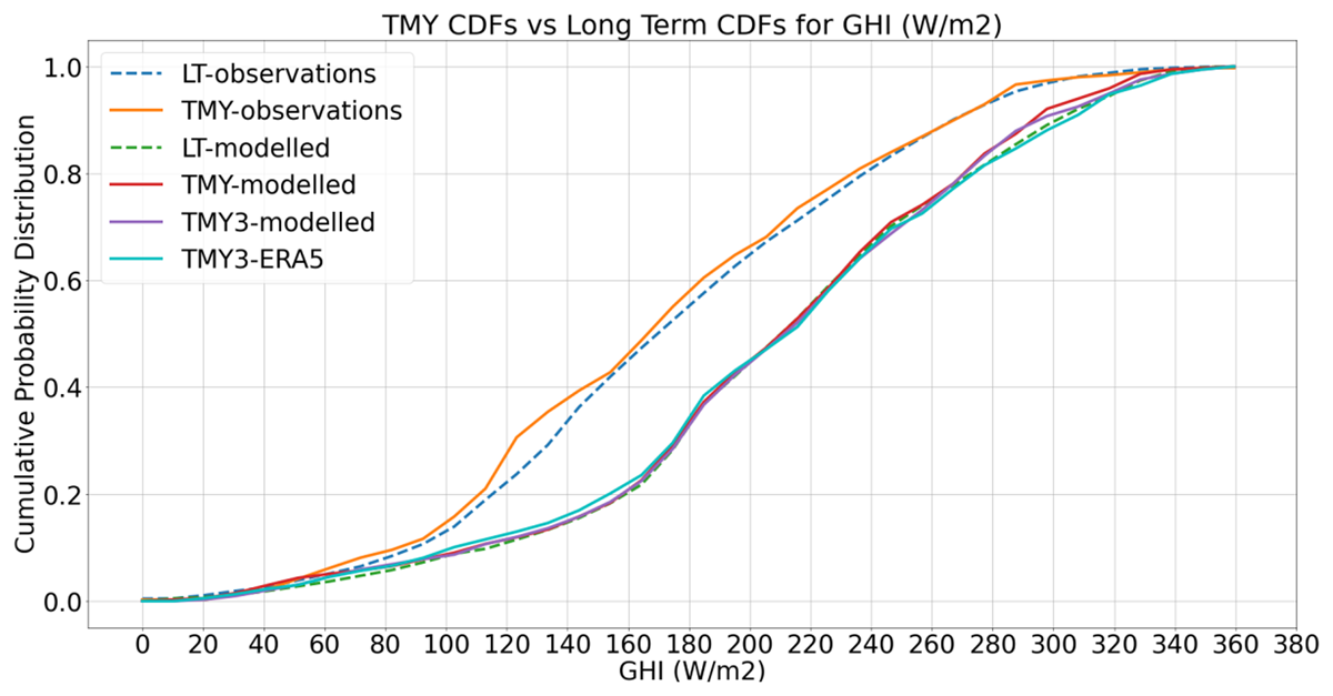
Figure 3
Comparison of the long-term average CDF and TMY CDFs for observed and modelled GHI.
South: Santa Maria/RS (A803)
For the Santa Maria station, there were at least 10 years from which TMM could be selected for each calendar month except for May, June, and July. For these months, there were only 9 years from which the TMM could be selected, yet this was deemed acceptable in the calculation of the TMY. The TMY was generated for each of the four different data sources and can be found in Table 5.
Table 5
The generated TMYs for different data sources, with the final FS statistic values for the TMY CDF compared to the long-term average CDF.
| MONTH | YEAR | |||
|---|---|---|---|---|
| TMYOBS | TMYMOD | TMY3MOD | TMY3REA | |
| January | 2007 | 2006 | 2006 | 2006 |
| February | 2013 | 2013 | 2013 | 2016 |
| March | 2014 | 2014 | 2014 | 2014 |
| April | 2011 | 2014 | 2014 | 2014 |
| May | 2015 | 2011 | 2011 | 2013 |
| June | 2010 | 2010 | 2010 | 2017 |
| July | 2016 | 2013 | 2013 | 2010 |
| August | 2008 | 2014 | 2014 | 2006 |
| September | 2012 | 2012 | 2015 | 2013 |
| October | 2016 | 2016 | 2016 | 2017 |
| November | 2013 | 2011 | 2005 | 2013 |
| December | 2016 | 2016 | 2016 | 2006 |
| FS | 0.0106 | 0.0049 | 0.0057 | 0.0047 |
From the generated TMYs, we can see that there is agreement of at least 2 of the data sources for every calendar month, with 1 month (March) having the complete agreement of the TMM.
Again, the CDF for each generated TMY is compared to the long term (LT) observed and modelled CDFs for the annual GHI, as shown in Figure 4. From this plot, we can see that there is a good agreement between the modelled and observed solar radiation at this location. Table 5 tabulates the Finkelstein-Schafer statistics for each TMY compared to its respective LT-CDF. It can be seen that this station had the lowest FS values of all the stations analyzed, with a 75% quartile value below 0.0069. However, the TS value for observational data was higher at this station.
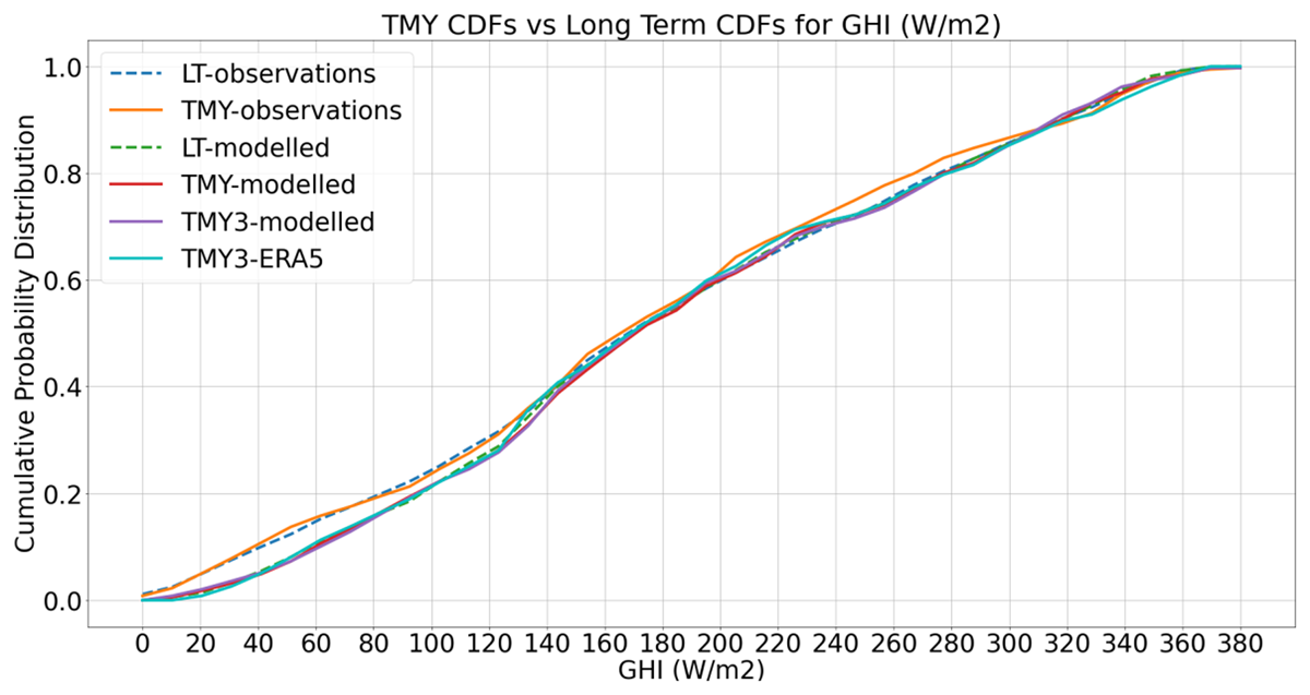
Figure 4
Comparison of the long-term average CDF and TMY CDFs for observed and modelled GHI.
North: Palmas/TO (A009)
For the Palmas station, there are at least 10 years from which the TMM can be selected available for each calendar month, except for November. There are 9 years of data available for November, and this is deemed acceptable considering the difficulty in obtaining 10 years of stable measurements for Northern Brazil. The TMY was generated for each of the four different data sources and can be found in Table 6.
Table 6
The generated TMYs for different data sources, with the final FS statistic values for the TMY CDF compared to the long-term average CDF.
| MONTH | YEAR | |||
|---|---|---|---|---|
| TMYOBS | TMYMOD | TMY3MOD | TMY3REA | |
| January | 2010 | 2007 | 2007 | 2017 |
| February | 2009 | 2012 | 2012 | 2012 |
| March | 2011 | 2011 | 2011 | 2015 |
| April | 2011 | 2011 | 2007 | 2013 |
| May | 2012 | 2007 | 2007 | 2011 |
| June | 2017 | 2015 | 2015 | 2013 |
| July | 2011 | 2011 | 2011 | 2011 |
| August | 2005 | 2011 | 2013 | 2016 |
| September | 2008 | 2008 | 2008 | 2012 |
| October | 2014 | 2016 | 2016 | 2014 |
| November | 2013 | 2006 | 2006 | 2006 |
| December | 2014 | 2010 | 2014 | 2014 |
| FS | 0.0076 | 0.0094 | 0.0092 | 0.0107 |
From the generated TMYs, we can see that there is agreement of at least 2 of the data sources for 11 calendar months, with 1 month (July) having the complete agreement of the TMM.The CDF for each generated TMY is compared to the long term (LT) observed and modelled CDFs for the annual GHI, as shown in Figure 5. From this plot, we can see that there is again a large discrepancy between the modelled and observed solar radiation at this location. In Table 6 the Finkelstein-Schafer statistic for each TMY compared to its respective LT-CDF are tabulated and the worst value was for the reanalysis data.
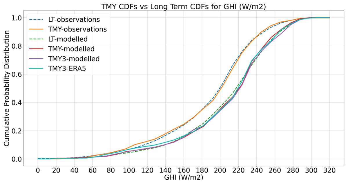
Figure 5
Comparison of the long-term average CDF and TMY CDFs for observed and modelled GHI.
Northeast: Caicó/RN (A316)
For the Caicó station, there are only 8 or 9 years from which the TMM can be selected for each calendar month. Once again, this is not ideal, yet considering the difficulty in obtaining long term stable measurements for Northern Brazil, this is acceptable for our generation of the TMY. The TMY was generated for each of the four different data sources and can be found in Table 7.
Table 7
The generated TMYs for different data sources for Caicó, with the final FS statistic values for the TMY CDF compared to the long-term average CDF.
| MONTH | YEAR | |||
|---|---|---|---|---|
| TMYOBS | TMYMOD | TMY3MOD | TMY3REA | |
| January | 2009 | 2008 | 2009 | 2009 |
| February | 2017 | 2008 | 2017 | 2012 |
| March | 2007 | 2015 | 2015 | 2014 |
| April | 2007 | 2007 | 2007 | 2007 |
| May | 2007 | 2013 | 2013 | 2017 |
| June | 2010 | 2010 | 2010 | 2010 |
| July | 2010 | 2014 | 2010 | 2010 |
| August | 2010 | 2010 | 2010 | 2014 |
| September | 2013 | 2010 | 2010 | 2015 |
| October | 2013 | 2014 | 2014 | 2014 |
| November | 2008 | 2008 | 2012 | 2016 |
| December | 2011 | 2007 | 2007 | 2012 |
| FS | 0.0085 | 0.0060 | 0.0069 | 0.0107 |
From the generated TMYs, we can see that there is agreement of at least 2 of the data sources for every calendar month, with 2 months (April and June) having the complete agreement of the TMM.
The CDF for each generated TMY is compared to the long term (LT) observed and modelled CDFs for the annual GHI, as shown in Figure 6. From this plot, we can see that there is only a slight discrepancy between the modelled and observed solar radiation at this location, but not as large as at other locations. In Table 7 the Finkelstein-Schafer statistic for each TMY compared to its respective LT-CDF are tabulated and the worst value was for the reanalysis data.
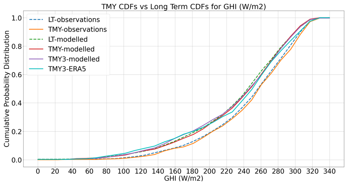
Figure 6
Comparison of the long-term average CDF and TMY CDFs for observed and modelled GHI.
From the TMYs generated for each of the 5 regions of Brazil, we can draw 4 main conclusions:
There is agreement in the TMMs between at least 2 data sources for at least 10 months for each region. This suggests that the typicality of the months is overall quite consistent, even if the data source is different.
Stations A001 and A803 have similar CDFs between observed/modeled and TMY/LT data, so they are not sensitive to data source selection. Although the TMMs may be slightly different, the overall CDF of the TMY is still very close to the LT. This is also reflected by the lowest FS values among all five stations studied.
For the A707, A009 and A316 stations there is discrepancy between the CDFs for observations and modelled data, meaning TMY may be sensitive to selection of data source at these locations. Table 8 shows the number of TMMs in agreement between TMYobs and any of the TMYs calculated from modelled data for each station. Table 8 shows essentially no correlation between stations that have discrepancy between observed and modelled data and agreement in TMMs. Whilst the A707 station (which had a large discrepancy between modelled and observed data) only has three months in agreement, the A009 station which also had a large discrepancy has 6 months in agreement. This suggests that whilst the discrepancy of the data will be important in the generated TMY dataset, the choice of which months are the most typical is not greatly affected. These stations presented the highest FS values among the stations studied.
The stations A803 and A707 have shown the worst results compared with the observations (Figures 3 and 4, respectively). This is also reflected in the greater discrepancy in FS. The reason for it is due to the influence of the ENSO events of the dataset. It is well known that ENSO is very well (and positively) correlated with the south part of Brazil (which is represented by the station A803) while this is not so clear for the southeast Brazil (represented by the station A707). So, the presence of this event (ENSO) can modify the shape of the curve (e.g., Figure 3) and the difference between the input data (Figure 4).
Table 8
Number of TMMs in agreement between TMYobs and TMYmod/TMY3mod/TMY3rea for each station.
| STATION | TMMs IN AGREEMENT | FS (75% QUARTILE) |
|---|---|---|
| Brasilia (A001) | 5 | 0.0078 |
| Pres. Prudente (A707) | 3 | 0.0101 |
| Sta Maria (A803) | 7 | 0.0069 |
| Palmas (A009) | 6 | 0.0097 |
| Caicó (A316) | 7 | 0.0091 |
To investigate this further, we could look at individual monthly CDFs, as opposed to the yearly CDF, as well as considering the ranking of the selected TMMs.
Weighting Sensitivity
In order to determine the sensitivity of our TMY generation procedure to the weighting scheme selected, we repeat the generation of the A001 TMY using observational data with the different weighting schemes found in Table 9. The resultant TMYs can be found in Table 10, alongside the most frequently occurring TMM for each calendar month.
Table 9
Weighting schemes used for calculating the TMY (in parts out of 24).
| SCHEME | T:RH:W:GHI | TMAX | TMIN | T | RHMAX | RHMIN | RH | WMAX | W | GHI |
|---|---|---|---|---|---|---|---|---|---|---|
| A | 4:4:4:12 | 1 | 1 | 2 | 1 | 1 | 2 | 2 | 2 | 12 |
| B | 2:2:2:18 | 1/2 | 1/2 | 1 | 1/2 | 1/2 | 1 | 1 | 1 | 18 |
| C | 0:0:0:24 | 0 | 0 | 0 | 0 | 0 | 0 | 0 | 0 | 24 |
| D | 6:6:6:6 | 3/2 | 3/2 | 3 | 3/2 | 3/2 | 3 | 3 | 3 | 6 |
| E | 0:8:8:8 | 0 | 0 | 0 | 2 | 2 | 4 | 4 | 4 | 8 |
| F | 8:0:8:8 | 2 | 2 | 4 | 0 | 0 | 0 | 4 | 4 | 8 |
| G | 8:8:0:8 | 2 | 2 | 4 | 2 | 2 | 4 | 0 | 0 | 8 |
| H | 8:8:8:0 | 2 | 2 | 4 | 2 | 2 | 4 | 4 | 4 | 0 |
Table 10
TMMs for Different Weighting Schemes, with TMMs different from the mode in italics.
| MONTH | TMY FOR DIFFERENT WEIGHTING SCHEMES | ||||||||
|---|---|---|---|---|---|---|---|---|---|
| A | B | C | D | E | F | G | H | TMM (MODE) | |
| January | 2009 | 2009 | 2017 | 2009 | 2008 | 2009 | 2009 | 2009 | 2009 |
| February | 2011 | 2011 | 2009 | 2011 | 2009 | 2009 | 2011 | 2011 | 2011 |
| March | 2013 | 2013 | 2013 | 2013 | 2013 | 2012 | 2013 | 2013 | 2013 |
| April | 2008 | 2008 | 2014 | 2008 | 2012 | 2014 | 2008 | 2008 | 2008 |
| May | 2017 | 2017 | 2017 | 2017 | 2017 | 2017 | 2017 | 2017 | 2017 |
| June | 2011 | 2011 | 2015 | 2011 | 2011 | 2011 | 2011 | 2011 | 2011 |
| July | 2013 | 2013 | 2013 | 2013 | 2013 | 2013 | 2013 | 2013 | 2013 |
| August | 2015 | 2015 | 2015 | 2015 | 2015 | 2015 | 2015 | 2015 | 2015 |
| September | 2014 | 2014 | 2014 | 2014 | 2014 | 2014 | 2012 | 2012 | 2014 |
| October | 2016 | 2016 | 2016 | 2016 | 2013 | 2016 | 2016 | 2016 | 2016 |
| November | 2014 | 2014 | 2014 | 2017 | 2008 | 2017 | 2014 | 2017 | 2014 |
| December | 2017 | 2017 | 2006 | 2017 | 2017 | 2017 | 2017 | 2017 | 2017 |
| Number different from mode | 0 | 0 | 5 | 1 | 5 | 4 | 1 | 2 | – |
From this table, we can see that we have the greatest variation from the mode for weighting schemes C, E and F. Scheme C corresponds to 100% weighting on the global radiation, scheme E corresponds to 0% weighting on the air temperature with equal weightings on the other indices, and scheme F corresponds to 0% weighting on the relative humidity, again with equal weighting on the other indices.
Even in these extreme cases, over half of the TMY still consists of the modal TMMs, suggesting that moderate changes in weighting schemes have very little effect on the TMY. Additionally, if we look the 3 lowest weighted sums of FS statistics for the extreme weighting scheme C, as one example shown in Table 11, we observe that in every case where the selected TMM is not the same as the mode, the mode is within the top 3 candidates. Again, this suggests that whilst the selected TMM may be different from the mode, the TMM is still very close to the long-term average and therefore the resultant TMY time series will not be significantly different.
Table 11
The months with the 3 lowest weighted sums of the FS statistic (×10–3), using weighting scheme C.
| YEAR | JAN | FEB | MAR | APR | MAY | JUN | JUL | AUG | SEP | OCT | NOV | DEC |
|---|---|---|---|---|---|---|---|---|---|---|---|---|
| 2005 | – | – | – | – | – | – | – | – | – | – | – | – |
| 2006 | – | – | – | – | – | – | – | – | – | – | 3.91 | 4.23 |
| 2007 | – | – | – | 3.57 | – | – | 4.62 | – | – | – | – | – |
| 2008 | – | – | – | 3.89 | – | – | – | 2.77 | – | – | – | – |
| 2009 | 4.52 | 4.04 | 4.08 | – | – | – | – | – | – | – | 3.54 | – |
| 2010 | 5.30 | – | – | – | 3.83 | – | – | – | – | 5.24 | – | 5.32 |
| 2011 | – | 4.27 | – | – | – | 2.91 | 3.82 | – | – | – | – | – |
| 2012 | – | – | 4.31 | – | – | 3.09 | – | 2.68 | 4.14 | – | – | – |
| 2013 | – | – | 4.04 | – | – | – | 2.58 | – | – | 5.62 | – | – |
| 2014 | – | – | – | 3.52 | 4.31 | – | – | – | 2.64 | – | 3.23 | – |
| 2015 | – | 4.09 | – | – | – | 2.41 | – | 2.18 | – | – | – | – |
| 2016 | – | – | – | – | – | – | – | – | 5.47 | 3.18 | – | – |
| 2017 | 3.91 | – | – | – | 3.60 | – | – | – | – | – | – | 4.24 |
Interestingly, the TMYs generated from weighting schemes G and H only differ from the mode by one or two months. These schemes have zero weighting on the wind velocity and global radiation, respectively. This suggests that the resultant TMY is more sensitive to changes in the temperature and relative humidity weightings than wind and global radiation. Overall, however, this investigation in the sensitivity to the weighting factors of the daily weather indexes has shown that so long as a moderate weighting scheme is selected, such as schemes A, B or D, the resultant TMY is not very different to the mode. TMMs which are not the mode are often from the top three candidates for a TMM, and therefore slight differences are not significant.
The resultant CDFs for the TMYs generated from each weighting scheme can be seen in Figure 7, demonstrating that even in the case of an extreme weighting scheme, the CDF is relatively unchanged from the long-term average. This investigation was done for the most extreme cases, therefore more moderate changes in the schemes are unlikely to have a significant effect, if any, on the resultant TMY, and therefore calculations with the weighting scheme used in this study are valid. This result suggests that the meteorological parameters used in this study to generate the TMY are well correlated and not independent variables, and therefore changing the weightings has little effect on the typicality of the month.
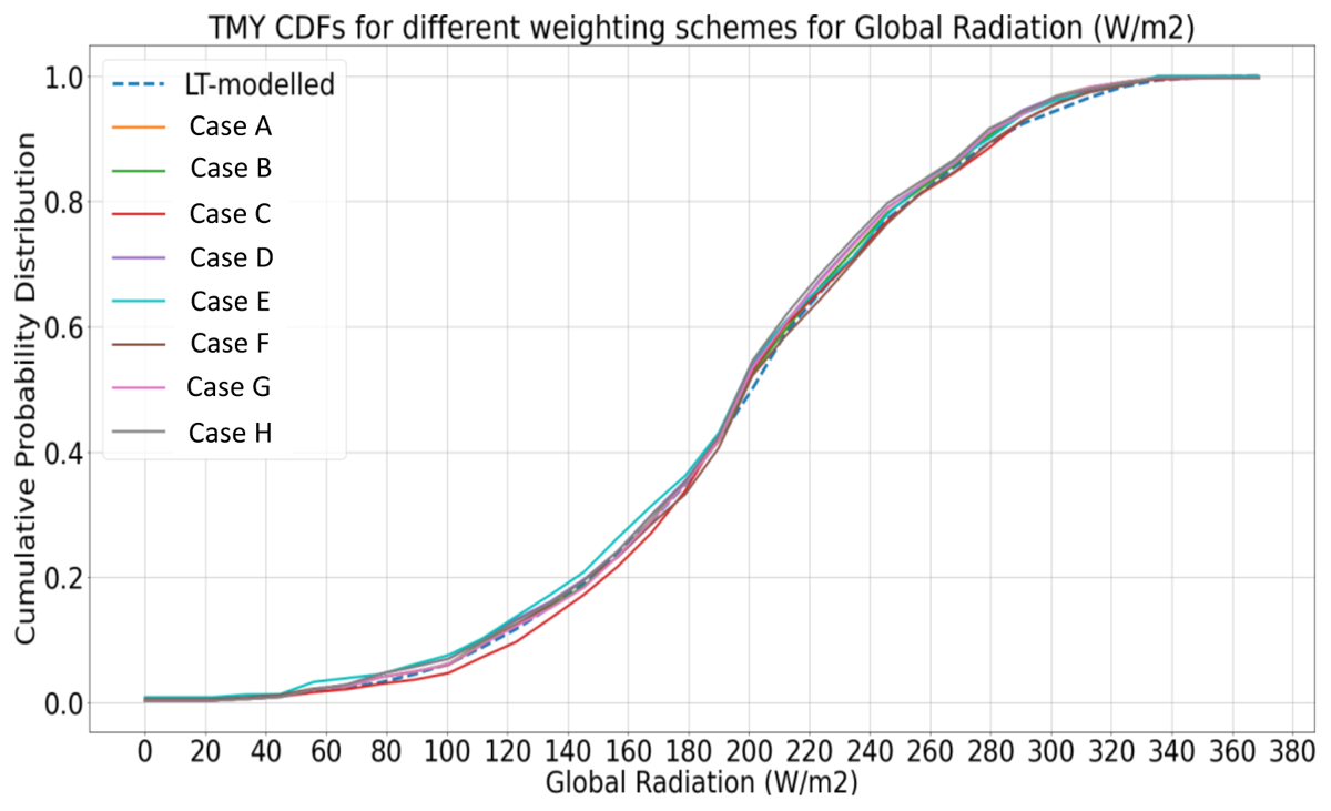
Figure 7
Comparison of the TMY CDFs for Global Horizontal Radiation for different weighting schemes at the A001 station.
Conclusions
In this study, a variation of the method proposed by Hall et al. (1978) was used to generate a dataset of typical meteorological years (TMY) for five representative climatic regions in Brazil. These TMYs were calculated from 13 years of meteorological data for 4 daily climate indices from three different sources: site-specific observations, modelled satellite data, and reanalysis data.
An examination of the sensitivity of the data sources revealed that the months identified as “most typical” by the methodology remain quite similar when different data sources are used. However, in cases where the data sources have very different values, the TMY result also contains different values depending on the data source, even when the months are the same. This suggests that the typicality of months is generally quite consistent, even when the data source is different. The discrepancy in the data is significant for the TMY dataset produced, but it does not significantly affect the choice of the most typical months.
The effects of changing the weighting factors of the meteorological parameters used to determine how typical a month is show that the final selection of the TMM is not very sensitive to extreme changes in the weighting factors. Therefore, the exact choice of the weighting scheme is relatively arbitrary, if not irrelevant, as long as it is moderate. This can be explained by the fact that the meteorological parameters used in this study are well correlated with each other and are not independent variables, so changing the weights has little effect on the typicality of the month. Therefore, to generate a TMY, only a few independent parameters are needed and using multiple interdependent parameters does not necessarily improve the quality of the generated TMY.
Data Accessibility Statement
The data used in the production of this article and which support the study’s conclusions are available upon request from the authors or can be obtained directly from the following data sources: http://labren.ccst.inpe.br/index-en.html; https://bdmep.inmet.gov.br.
Notes
Ethics And consent
The authors declare that this research does not involve any human subjects, human material or human data and that they do not violate any ethical precepts when submitting the material for publication.
Funding Information
Anna Tippet is grateful for the scholarship received from the Oxford University Summer Internship Program for her stay in Brazil at the National Institute for Space Research (INPE). The authors Enio Pereira and Fernando Martins thanks CNPq for their respective Research Grant processes 350023/2021-2 and 312929/2020-0. This work is also a contribution from the National Institute of Science and Technology for Climate Change (INCT-MC) funded by FAPESP 2014/50848-9, CNPq 465501/2014-1 and CAPES/FAPS nº 16/2014.
Competing Interests
The authors have no competing interests to declare.
Author contributions
Anna Tippet: survey, data processing and statistical calculations, creation of tables, figures, etc.
Enio Pereira: conception, research coordination and writing and review.
André Gonçalves: technical and scientific support and review.
Fernando Martins: technical and scientific support and review.
Gilberto Fisch: technical and scientific support and review.
Rodrigo Costa: technical and scientific support and review.