
1 Introduction
Operational data assimilation systems ingest large volumes of measurements from meteorological satellites. Especially in global applications of Numerical Weather Prediction (NWP), where the focus is generally in medium-range prediction capabilities, radiance sounders on polar-orbiting and geostationary platforms are among the most influential observing systems (e.g., Eyre et al. 2022). The radiance assimilation is commonplace in limited-area (regional) NWP systems too, albeit their relative importance in such applications tends to be less. The most common use case for radiance data is from sounders operating at microwave and infrared wavelengths (e.g., Kazumori, 2014; Lin et al., 2017; Lindskog, Dybbroe & Randriamampianina, 2021). By now, a mature status has been reached also in the area of using microwave imagers (e.g., Geer et al., 2022).
Successful assimilation of radiance data requires careful handling of observation error. Radiance observations in most cases include a non-negligible contribution from systematic errors. Such observation biases may originate directly from instrument-specific characteristics and sensor design or indirectly from data assimilation practicalities, such as inaccuracies in radiative transfer modelling or observation quality control process. In the context of radiance assimilation, the careful handling of errors implies explicit treatment to account for the observation bias, i.e., an application of a bias correction algorithm (Harris & Kelly, 2001; Auligné, McNally & Dee, 2007).
Data assimilation algorithms retrieve meteorological information from departures of observations from their forward-modelled counterparts computed from a short-range NWP forecast; these departures are sometimes called ‘innovations’ in the data assimilation terminology. Such departures may be affected by biases in either observations, the short-range forecast, or both. A well-designed bias correction scheme should allow for correcting for the observation bias only. Harris & Kelly (2001) proposed their parametric formulation with this particular goal in mind, and their scheme still constitutes the basis for modern, more advanced bias correction schemes. In practice, the bias correction is derived from a set of geometric and physical predictor variables and weights (bias correction coefficients) assigned to each of them. The predictors typically include observation and solar view angles, air-mass thicknesses in selected pressure level intervals, and skin temperature. The most advanced variational systems have demonstrated capability to routinely optimize the weighting of the predictors inside the data assimilation process (Auligné, McNally & Dee, 2007; Benáček & Mile, 2019).
Adaptive schemes such as the Variational Bias Correction (VarBC; Auligné, McNally & Dee, 2007) review and update the bias correction coefficients at all analysis hours in a cycled forecasting system. The coefficients are made part of the assimilation control vector so that the updates take place simultaneously with the estimation of all other analysis state variables. For the process to be robust and reliable, there needs to be a reasonably large sample of observations that represent the full range of predictor values. When considering state-of-the-art convective-scale regional models of today, the requirement of sufficiently heterogeneous sampling is not easily fulfilled. Furthermore, such high-resolution NWP systems often employ a frequent update cycle and relatively short assimilation time windows, implying that successive analyses are likely to have a highly variable coverage and data count from any given polar-orbiting satellite.
The Scandinavian-Baltic NWP group MetCoOp (Meteorological Co-operation on Operational NWP; Müller et al. (2017)) operates limited-area systems in convection-resolving scales. Figure 1 illustrates the large variability of satellite data coverage in their flagship operational product (MetCoOp Ensemble Prediction System; MEPS). The rectangle indicates the limited-area modelling domain and dots show locations of observations collected from one satellite instrument, that is the Advanced Microwave Sounding Unit -A (AMSU-A) of the Metop-C satellite. The data are shown at the synoptic analysis hours from 06 to 21 UTC on one day. There is no data inside the domain at 00 and 03 UTC (not shown). Also at 06 and 15 UTC (panels (a) and (d)), the coverage is poor and there are only a few data points close to the lateral boundaries. The data coverage is arguably sufficient for useful assimilation from descending-node overpasses at 09 and 12 UTC (panels (b) and (c)) and from ascending-node overpasses at 18 and 21 UTC ( (e) and (f)). At all analysis hours, the observation geometry differs substantially from both the previous and the following analysis. Given that Metop-C is in a maintained sun-synchronous orbit, the data coverage at each analysis hour is broadly similar on consecutive days.
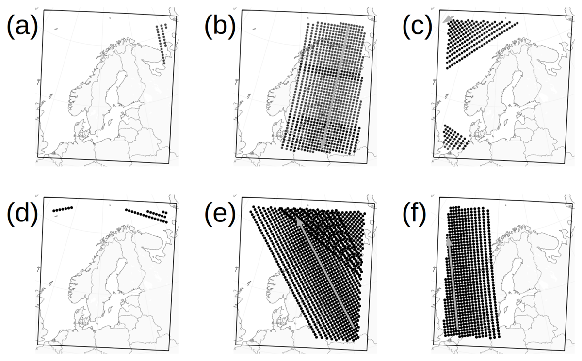
Figure 1
Example of satellite data coverage inside the MetCoOp NWP system domain. Dots indicate locations of the Advanced Microwave Sounding Unit -A (AMSU-A) observations from Metop-C satellite in three-hour time windows centred at synoptic times (a) 06, (b) 09, (c) 12, (d) 15, (e) 18, and (f) 21 UTC on 1 February 2023. Arrows indicate the approximate ground tracks of the satellite.
Considering the aspects of robustness and reliability in the adaptive bias correction process for the specific example shown in Figure 1, the representation of all possible predictor values is best guaranteed at 09 and 18 UTC. At these analysis hours, the ground track of the satellite (the gray arrow) aligns such that the full range of viewing angles is captured within the computing domain. At other analysis hours the data coverage is restricted to either left- or right-hand-side of the ground track so that the sampling of the view angles is non-exhaustive.
VarBC implementations in limited-area NWP systems have previously been discussed in a number of studies. Lin et al. (2017) reported no particular difficulty associated with the variations in data coverage, which suggests that the problem described above is specific to relatively small computing domain sizes. The solution suggested by Kazumori (2014) is to refrain from updating the bias correction coefficients inside the limited-area analysis, but instead employ coefficient values as they appear in the latest available analysis in a global NWP system. Randriamampianina, Iversen & Storto (2011) suggested cycling the VarBC coefficient information in 24-hour intervals and doing this separately at each daily analysis hour. This is a reasonably valid approach since the sun-synchronous satellites always provide approximately the same data coverage at 24-hour intervals. Benáček & Mile (2019) conducted a systematic comparison of the methods of Kazumori (2014) and Randriamampianina, Iversen & Storto (2011) and ended up suggesting the latter as more appropriate, largely because the selection of predictors in global NWP systems is not directly applicable to limited-area systems with relatively low model top.
In addition to the sun-synchronous satellite missions considered here, there are meteorological satellites in non-sun-synchronous low Earth orbits too. The methods discusses in this work are mostly not applicable to such satellites.
In this article, we propose an alternative approach to implementing VarBC in limited-area systems. In essence, we suggest to modify the daily update scheme of Randriamampianina, Iversen & Storto (2011) such that the coefficients get updated only at those analysis hours when the data coverage is expected to be sufficient for robust estimation. The underlying assumption is that such robust coefficients will be sufficiently representative of the data at other analysis hours too. We describe the proposal in a general sense in Section 2 and from the point of view of a specific application in the MetCoOp NWP systems in Section 3. Later, we present a performance evaluation of the proposed scheme in Section 4 and concluding remarks in Section 5.
2 Three Variants of VarBC
Variational data assimilation searches for the model state xa, also called the analysis, that minimizes the quadratic distance to the background xb on the one hand and to the observations y on the other. Mathematically, the problem is formulated in terms of the cost function J(x)
where x is the model state and matrices B and R are representations of stochastic error covariances in the background and observations, respectively. The operator H is the forward model (observation operator) that transforms the model state into observation space. The statistically optimal analysis is the model state that minimizes J, i.e.,
In the VarBC scheme, the bias correction coefficients β are made part of the model state vector. To highlight this aspect, the cost function is rewritten as
Here, the first term on the right-hand side is the same as in Eq. (1). The second term penalizes for the distance of the bias correction coefficients from their a priori values, denoted by βb. The error covariance associated to βb is accounted for in the matrix Bβ. The third term is the quadratic distance of the model state from observations, similar to the second term in Eq. (1), but with the additional dependency via the bias correction model .
The three VarBC variants discussed in this Section differ in terms of (i) where βb is taken from and (ii) whether β is allowed to deviate from βb at all analysis hours. In the simplest formulation in a cycled analysis-forecasting system, such deviations are allowed at all hours and , i.e., the first guess provided to the analysis at time j, equals , that is the state found optimal in the previous analysis time at j–1. Figure 2 is a schematic illustration of this variant, that we call “Single Stream Continuous Update” (SSCU) in this article. The cycling of βb goes at the regular cycling interval together with xb. This variant is best suited for use in global systems where there is a solid and reliable stream of observations from all satellite instruments at all analysis hours.
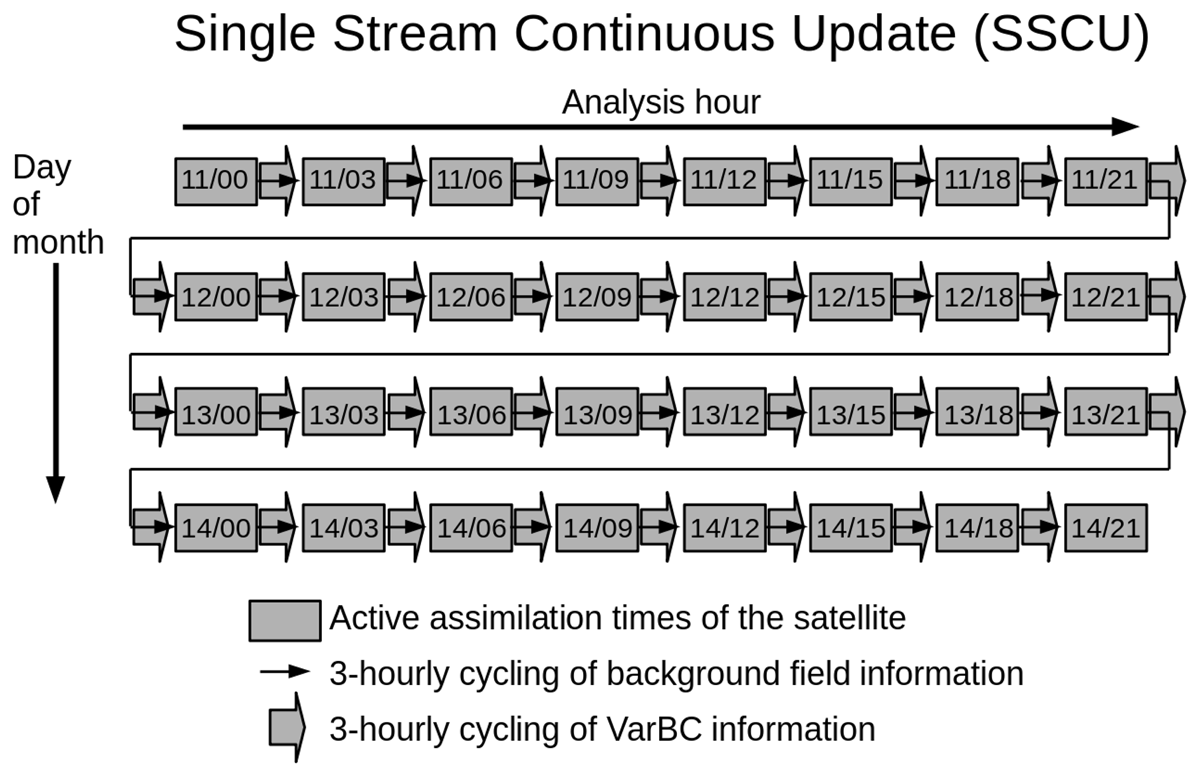
Figure 2
Cycling of VarBC coefficients in the Single Stream Continuous Update variant.
The SSCU variant performs poorly in convective-scale limited-area systems of today (Randriamampianina, Iversen & Storto, 2011; Kazumori, 2014; Benáček & Mile, 2019). Although VarBC algorithms (by design) are sufficiently flexible to take account of how the number of available observations varies from one analysis time to another, they cannot easily deal with scenarios where the sampling of predictors is irregular. Robust estimation of the bias correction coefficients requires that the range of predictor values is fully represented in the data, but this is generally not the case in limited-area systems such as the one illustrated in Figure 1.
In the context of the ACCORD (A Consortium for Convective-scale modelling Research and Development) consortium, comprising 26 meteorological offices from Europe and Mediterranean countries, most operational VarBC implementations follow the proposal of Randriamampianina, Iversen & Storto (2011). Figure 3 is a schematic representation of this variant that we call “Multiple Stream Daily Update” (MSDU). The provision of βb is detached from the regular analysis-to-forecast cycling and instead taken from the state found optimal 24 hours earlier. Since the meteorological satellites in question here are in sun-synchronous orbits, the observation coverage is broadly similar at 24-hour intervals, so the previously updated coefficients can be considered reasonably representative of the situation at hand. From any given satellite, data can still be assimilated several times daily, but there is no communication between the bias correction coefficients representative of different analysis hours.
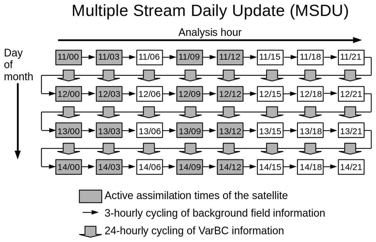
Figure 3
Cycling of VarBC coefficients in the Multiple Stream Daily Update variant.
The MSDU variant allows one to maintain independent streams of VarBC coefficients even at hours when no active assimilation is carried out (shown by the white rectangles in Figures 3, 4). This is useful when a previously maintained satellite has started to drift in its orbit and the data coverage at a given analysis hour is slowly evolving over time. The analysis hours at which active assimilation is performed may then require reconsideration from time to time.
For now, we believe that MSDU is the best working solution in the operational domains within the ACCORD consortium. However, the method comes with certain unattractive properties that we list as follows:
In operational context there often are other (non-satellite) observation types that also require bias correction and may be poorly-suited for the 24-hour cycling. Atmospheric Path Delay (APD) data processed from ground-based receiver networks of Global Navigation Satellite Systems (GNSS) is an example of such an observation type (Sánchez Arriola et al. 2016). It is a significant technical burden to maintain several VarBC cycling intervals in parallel.
It can take a long time to mature the VarBC coefficients at those analysis hours when data coverage inside the limited-area modelling domain is partial (such as 12 and 21 UTC in the case of Metop-C in the MetCoOp domain; see Figure 1). This will increase the time it takes to start active use of new instruments, and there is a risk of reduced usability of data after sudden changes in instrument measurement characteristics.
The observation minus background departures may contain systematic model-driven diurnal variations that the bias correction scheme struggles to distinguish from observation biases. It will be difficult to detect such diurnal patterns in multiple independent streams of bias-corrected data, and such patterns will likely be present in analyses too.
Our proposed modification to the MSDU scheme is illustrated in Figure 4. We call this variant “Single Stream Daily Update” (SSDU). Here, the cycling of βb goes along with the regular cycling interval, so it is sufficient to maintain only a single stream of VarBC coefficients that is considered valid at all analysis hours. Crucially though, coefficient updates are allowed only once per day for any given satellite instrument. The idea is to choose the analysis hour for the update separately for each satellite in a way that accounts for the expected data coverage and maximizes sampling of the full range of predictor values. This setup will avoid the unattractive characteristics of MSDU described above. However, SSDU is unable to account for possible diurnal variations in the observation biases, which may become a disadvantage in some circumstances.
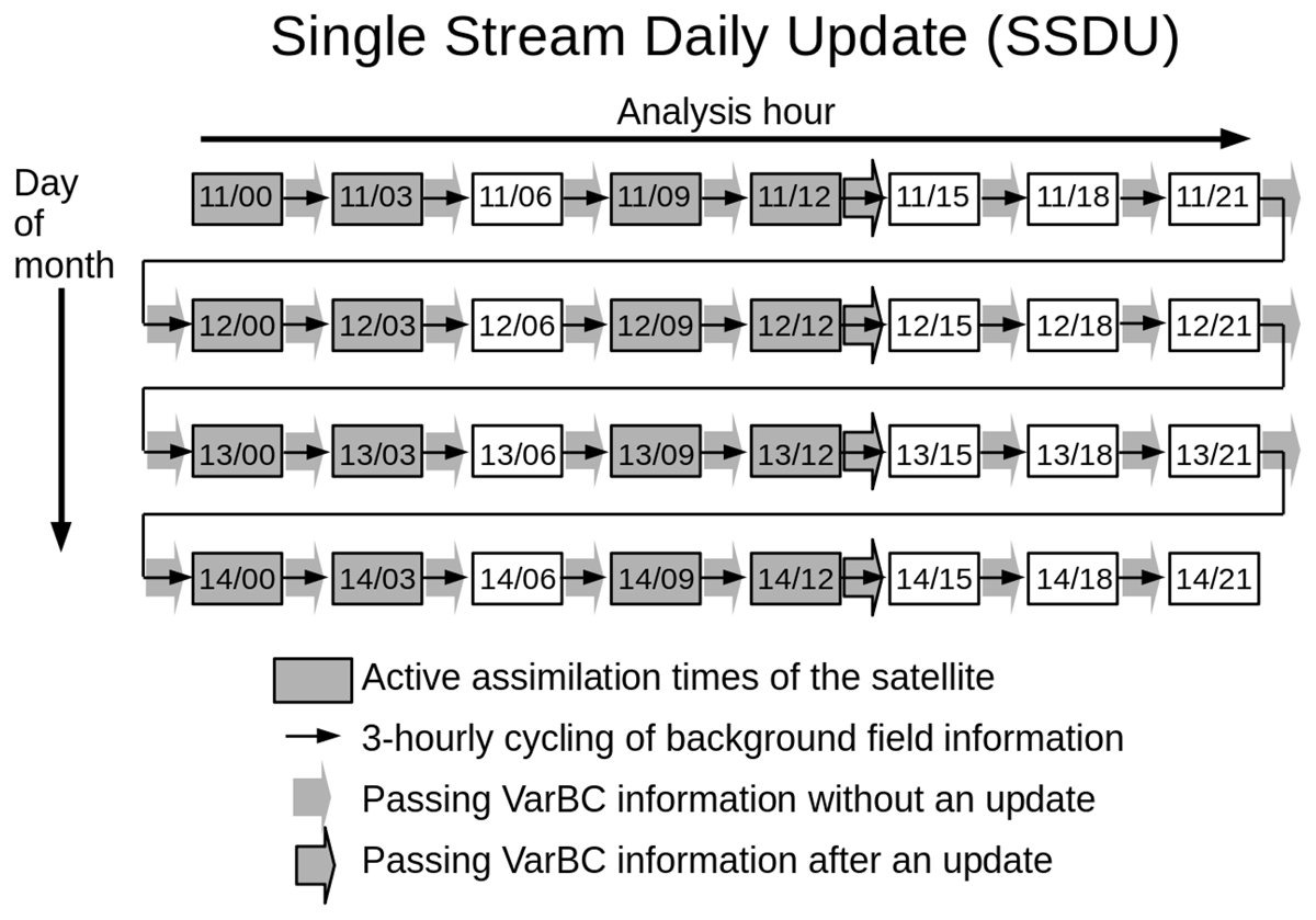
Figure 4
Cycling of VarBC coefficients in the Single Stream Daily Update variant.
3 A Proposal on Implementation of SSDU at MetCoOp
3.1 The MetCoOp operational suites
The operational NWP systems at MetCoOp (Müller et al. 2017) apply 2.5 km horizontal grid spacing in the domain shown in Figure 1. In vertical, the grid applies a terrain-following hybrid coordinate system of 65 levels. The lowest level is at the height of 12 meters and the highest is at 10 hPa pressure. Each forecast is initialized to an analyzed model state as obtained through three-dimensional variational data assimilation (3D-Var) and optimal interpolation (OI), respectively for the analyses of upper-air and surface variables. Lateral boundary forcing in one-hour resolution is taken from a global host model forecast, that comes from the operational NWP system of the European Centre for Medium-range Weather Forecasts (ECMWF). The ECMWF forecast data is also made use of through the so-called large-scale mixing process, that incorporates planetary scale information into the background field just before the data assimilation (Dahlgren & Gustafsson, 2012).
The numerical code base for the MetCoOp NWP systems comes from international collaboration effort taken within the High Resolution Limited Area Model (HIRLAM), Aire Limitée Adaptation dynamique Développement International (ALADIN), and ACCORD consortia. Operational suites are built on top of reference versions of the HIRLAM-ALADIN Research on Mesoscale Operational NWP in Euromed – Applications of Research to Operations at Mesoscale (HARMONIE-AROME) system (Bengtsson et al. 2017). Since March 2021, these operational suites have been based on the HARMONIE-AROME reference cycle 43.
3.1.1 MetCoOp Ensemble Prediction System (MEPS)
MEPS is the primary operational NWP system at MetCoOp and it provides an hourly-updating ensemble forecast with maximum lead time at 66 hours. The MEPS analysis takes the background field from an earlier three-hour forecast (i.e., the cycling interval is three hours). The data assimilation considers the following observation types: (1) synoptic observations at surface stations and ships, (2) drifting buoys, (3) radiosondes, (4) aircrafts, (5) APD from ground-based GNSS receiver networks, (6) reflectivities and Doppler winds from ground-based meteorological radars, and (7) polar-orbiting satellite data from instruments including the Advanced Microwave Sounding Unit -A (AMSU-A), Advanced Scatterometer (ASCAT), Advanced Technology Microwave Sounder (ATMS), Cross-track Infrared Sounder (CrIS), Infrared Atmospheric Sounding Interferometer (IASI), Micro-Wave Humidity Sounder –2 (MWHS-2), and Microwave Humidity Sounder (MHS). Time selection is applied to all satellite observations to avoid attempting to use data at analysis times when data coverage is poor, because no robust bias correction information is available at such times.
The MEPS ensemble consists of a deterministic and 14 perturbed members. Stochastic perturbations are introduced to lateral boundary forcing, observations, analysed model state, and certain parameters in model physics description as documented in Frogner et al. (2019) and Frogner et al. (2022). The ensemble is distributed in time such that five new members are launched every hour. The deterministic (unperturbed) member and four perturbed members run at the synoptic analysis hours (hereafter S0 hours: 00, 03, 06, 09, 12, 15, 18, and 21 UTC). The other 10 perturbed members are distributed evenly between the one-hour offset (hereafter S1 hours: 01, 04, 07, 10, 13, 16, 19, and 22 UTC) and two-hour offset (hereafter S2 hours: 02, 05, 08, 11, 14, 17, 20, and 23 UTC) with respect to the synoptic hours.
3.1.2 MetCoOp Nowcasting System (MNWC)
MetCoOp also maintains a separate operational NWP suite designed for use in forecasting at very short lead times, i.e., nowcasting. The MetCoOp Nowcasting System (MNWC) differs from MEPS in the following aspects:
Forecast lead time is restricted to 12 hours.
There is no ensemble of forecasts but only the deterministic unperturbed run.
New unperturbed analysis and forecast are produced every hour.
Assimilation time window is one hour (centred at each full hour).
There is no internal forecast-to-analysis cycling. Instead, the MNWC analysis takes the background field from the deterministic MEPS forecast (at either 3-, 4-, or 5-hour lead time depending on the analysis time).
The cut-off time for observations is 25 minutes past the analysis time (in contrast with 75 minutes as in MEPS). This means using fewer observations in general, although the use of various observation types is the same as in MEPS.
There is an additional step towards improving the consistency of cloud analysis with geostationary satellite imagery as described in Gregow et al. (2020).
The HARMONIE-AROME code base, as well as majority of settings applied in the use of observations, data assimilation, forecast model physics and numerical aspects are identical between MEPS and MNWC suites.
3.2 SSDU update hours in MEPS and MNWC
Each polar orbiter makes five or six daily overpasses of significance over the MetCoOp operational domain. As an example, the NOAA-20 and S-NPP satellites provide a substantial amount of data for use in the MEPS analyses at 00–05 and 08–13 UTC every day. The analysis hours of active assimilation with these satellites are indicated for the deterministic member by the shaded rectangles in Figures 2, 4. As illustrated in Figure 3, the currently-used implementation of MSDU maintains eight independent streams of VarBC coefficients. To replace the MSDU implementation by one based on SSDU, one will need to specify the hour of daily coefficient update separately for each satellite. Furthermore, the daily update hours are needed separately for ensemble members running at S0, S1, and S2 hours. To choose the most appropriate update hours, we consider the typical availability of data inside the MetCoOp domain at different analysis hours. At the ideal update hour, there will be data from all scan positions and also the sampling of other VarBC predictors (i.e., air-mass thicknesses) is as comprehensive as possible. In our view, this will be the best guarantee for robust and reliable VarBC performance.
It is obvious that the time of the most comprehensive data availability depends on satellite orbit parameters, but it will also depend heavily on the limited-area modelling domain. For a practical application specifically in the MetCoOp domain, we apply subjective selection based on frequency distributions of data collected from each scan position at each analysis hour. Figure 5 is an illustration of the method and represents the cases of NOAA-20 ATMS and Metop-C AMSU-A as they appeared in August 2021. NOAA-20 and Metop-C are particularly illustrative since they are in maintained orbits and highlight typical data coverage that can be expected from satellites in the so-called afternoon and morning orbits. The accumulated data count is shown separately for each analysis hour and those falling into either S0, S1, or S2 hours are arranged in separate panels. As expected, all panels demonstrate a considerable variation in the sampled frequency distribution. It is not at all common to have uniform sampling across the range of scan positions. In the case of NOAA-20 (panels (a)–(c)), the sampling is reasonably uniform at 12 UTC and at 02 UTC. These are the ideal VarBC update hours for members running at S0 and S2 hours, respectively. For members running at S1 hours, the choice is not obvious, although the distribution at 01 UTC is perhaps the least non-uniform in this case. Applying the same criteria for Metop-C (panels (d)–(f)), the sampling distributions are most comprehensive across the scan positions at 09, 19, and 20 UTC.
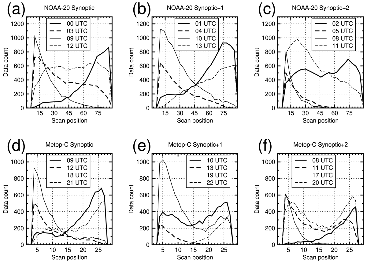
Figure 5
Frequency distributions of data count collected at different scan positions in August 2021. Panels (a)–(c) are for NOAA-20 ATMS and panels (d)–(f) for Metop-C AMSU-A. Thick solid, thick dashed, thin solid, and thin dashed lines indicate the data at different analysis hours in members run at S0, S1, and S2 hours, as shown in the legends.
The daily VarBC update hours that we suggest for adoption in all MEPS members are given in Table 1. The hours are provided for those satellites that are currently in operational use. The hours will need to be adjusted from time to time for those satellites that are in drifting orbits (i.e., NOAA-18 and NOAA-19 at the time of writing). The orbit information shown in the table corresponds to the situation in August 2021.
Table 1
The proposed daily update hours at MetCoOp NWP suites.
| SATELLITE | S0 | S1 | S2 |
|---|---|---|---|
| NOAA-18 | 12 UTC | 19 UTC | 20 UTC |
| NOAA-19 | 06 UTC | 07 UTC | 17 UTC |
| S-NPP | 12 UTC | 01 UTC | 02 UTC |
| NOAA-20 | 12 UTC | 01 UTC | 02 UTC |
| FengYun-3D | 12 UTC | 01 UTC | 02 UTC |
| Metop-B | 09 UTC | 19 UTC | 20 UTC |
| Metop-C | 09 UTC | 19 UTC | 20 UTC |
The implementation in the MNWC suite is slightly different because the system operates at one-hourly update interval and the data assimilation time window is just one hour. Since the time window is considerably shorter than the orbital period of the polar-orbiting satellites (that is, one hour and 40 minutes), each daily analysis hour will be populated by data from a given satellite only up to 60% of days. Consequently, selecting one analysis hour for the daily update will result in frequently missing the chance to actually make the update. Our proposed solution is to allow up to three daily updates in MNWC. The analysis times of the potential updates are chosen to be the same as those selected for the S0, S1, and S2 hours in the proposed implementation in MEPS.
4 Performance Evaluation of SSDU Against MSDU
4.1 Experiment setup
Following basic technical testing of the proposed new functionality, the SSDU scheme has been implemented as a non-default option in the most recent reference version of the HARMONIE-AROME system (Cy43h2.2). We have conducted a more thorough evaluation of the setup in a numerical experiment that is broadly similar to the operational design of MEPS. The experiment is run using the high-performance computing facilities of ECMWF and it consists of three independent parallel components. Each component comprises a control run based on the MSDU variant and a test run based on SSDU. The setup of the SSDU scheme is as detailed in previous section. The three components mimic the practice to launch different MEPS members at different analysis hours. However, the ensemble perturbations are left out of consideration and thus all experiment runs are to be considered deterministic. The runs are based on the version Cy43h2.1 of the HARMONIE-AROME reference system. In terms of the use of novel observation types such as radar reflectivities, scatterometer winds, and satellite radiances, the experiment runs follow the operational practice as it stood in late 2021 at MetCoOp. Throughout the experiment, we use the MetCoOp domain and take lateral boundary forcing from global forecasts provided by ECMWF.
All the runs are started on 1st August and continued until 15th September 2021. At the start, the VarBC coefficients are initialized to the state determined by another (in broad terms similar but independent) experiment that had been run earlier and covered from late May to the end of July 2021. This experiment applied three-hour cycling (only at S0 hours) and the VarBC information was updated according to the MSDU scheme. The control run at S0 hours takes the initial VarBC information directly as it appears at the end of the independent experiment. The control runs at S1 and S2 hours initialize the VarBC coefficients to the preceding S0 hour (that is, the initial VarBC coefficients at 01 and 02 UTC are the same as at 00 UTC, those at 04 and 05 UTC are the same as at 03 UTC, and so on).
Also the SSDU test runs initialize their VarBC coefficients to the state determined by the independent run at the end of July 2021. However, manual intervention is made such that the coefficients assigned to each satellite at 00 UTC on 1st August match those updated at the relevant analysis hour on the last day of the independent run. For instance, the SSDU test run at S0 hours initializes the coefficients for NOAA-20, S-NPP, and FY-3D to the state updated at 12 UTC, while it initializes the coefficients for Metop-B and Metop-C to the state updated at 09 UTC. The initial coefficients at 00 UTC on 1st August are copied as such to the other two test runs started at 01 and 02 UTC.
Since the the initial VarBC coefficients at S0 hours have had more than two months to adjust in the independent run, we consider them appropriate as such for serious experimenting. However, the initial coefficients at S1 and S2 hours may not be that representative of the actual assimilation hours, which is why we apply an additional 10-day warming-up period to allow for better adjusting to the actual analysis hours. Consequently, the data fit and forecast evaluations presented below (sections 4.2.2–4.2.4) are all based on the 36-day period from 11th August to 15th September 2021.
4.2 Results
4.2.1 Time series of mean observation minus background (O-B) departure
As the first diagnostic, we consider the time series of mean O-B departure as shown in Figure 6 for the full extent of the 46-day experiment. The figure shows representative examples of channel behaviour in temperature-sounding channels at microwave frequencies (panels (a) and (b)), a humidity-sounding channel at microwave frequencies (panel (c)), and a temperature-sounding channel at infrared frequencies (panel (d)). Timestep index on the x-axis goes from 1 to 1104 including all full hours from 00 UTC on 1st August to 23 UTC on 15th September 2021. The data is stratified such that the S0, S1, and S2 hours are shown respectively at the top, middle, and bottom part of each panel (a)–(d).
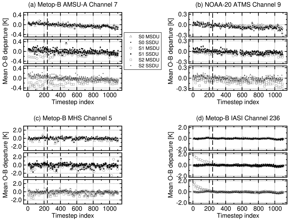
Figure 6
Time series of mean observation minus background (O-B) departure in representative sounder channels. (a) Channel 7 of Metop-B AMSU-A, (b) channel 9 of NOAA-20 ATMS, (c) channel 5 of Metop-B MHS, and (d) channel 236 of Metop-B IASI. In each panel, the data at S0, S1, and S2 hours are shown at the top, middle, and bottom, respectively. Data of the control runs are shown by triangles, circles and squares; that of the test runs by dots, diamonds and asterisks. The thick dashed line indicates the start of the 36-day evaluation period.
At the S0 hours, the behaviour of the mean O-B departure shows only little difference between the control and test runs. In the humidity sounding channel at microwave (Figure 6c), there is a weak signal of mean O-B going occasionally close to -1.0 K while it usually stays within ±0.5 K. The outliers occur mostly in the control run at either 12 or 21 UTC analysis. These analysis hours sometimes suffer from relatively low data numbers from the Metop-B satellite. At S1 and S2 analysis hours, there is a stronger signal in temperature-sounding channels at both microwave and infrared frequencies. There are numerous cases of the control run (circles and squares) failing to provide a good O-B fit. This is particularly obvious in the infrared channel (Figure 6d) at the beginning of the time series. The fit, however, becomes seemingly good by the time the 36-day evaluation period kicks in (marked by the thick dashed lines), so we assume this to be associated to the sub-optimal use of the S0 hour data when initializing the VarBC coefficients at the start of the experiment. In the temperature-sounding channels in microwave regime (panels (a) and (b)), the control run suffers from occasional poor fit throughout the evaluation period. The test runs applying the SSDU scheme do not reveal many such failures in the O-B fit.
4.2.2 Aggregated O-B departure statistics in radiance data
The next diagnostic to consider is the O-B fit in the radiance data as aggregated over the whole of the 36-day evaluation period. Figures 7 and 8 show the mean and standard deviation of the O-B departure in microwave sounder channels of NOAA-20 and Metop-C satellites (respectively). In both figures there are 12 panels corresponding to the daily analysis hours that include assimilation of the instrument data in question. The panels are arranged such that the S0, S1, and S2 hours go to the top, middle, and bottom rows, respectively. Furthermore, panels (a), (e), and (i) correspond to the analysis hours doing the daily update in the SSDU scheme.
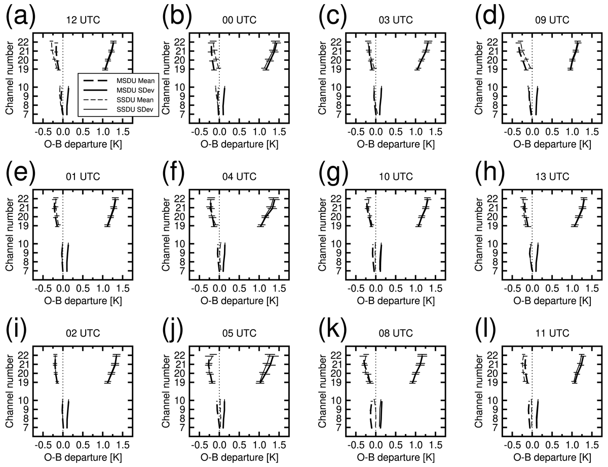
Figure 7
Observation minus background (O-B) departure statistics in the actively-assimilated channels of NOAA-20 ATMS. Control and test runs are shown by thick and thin lines, respectively. Dashed and solid lines represent mean and standard deviation. Bars indicate the 95% confidence intervals. The different panels indicate data at different analysis hours as shown in the headings.
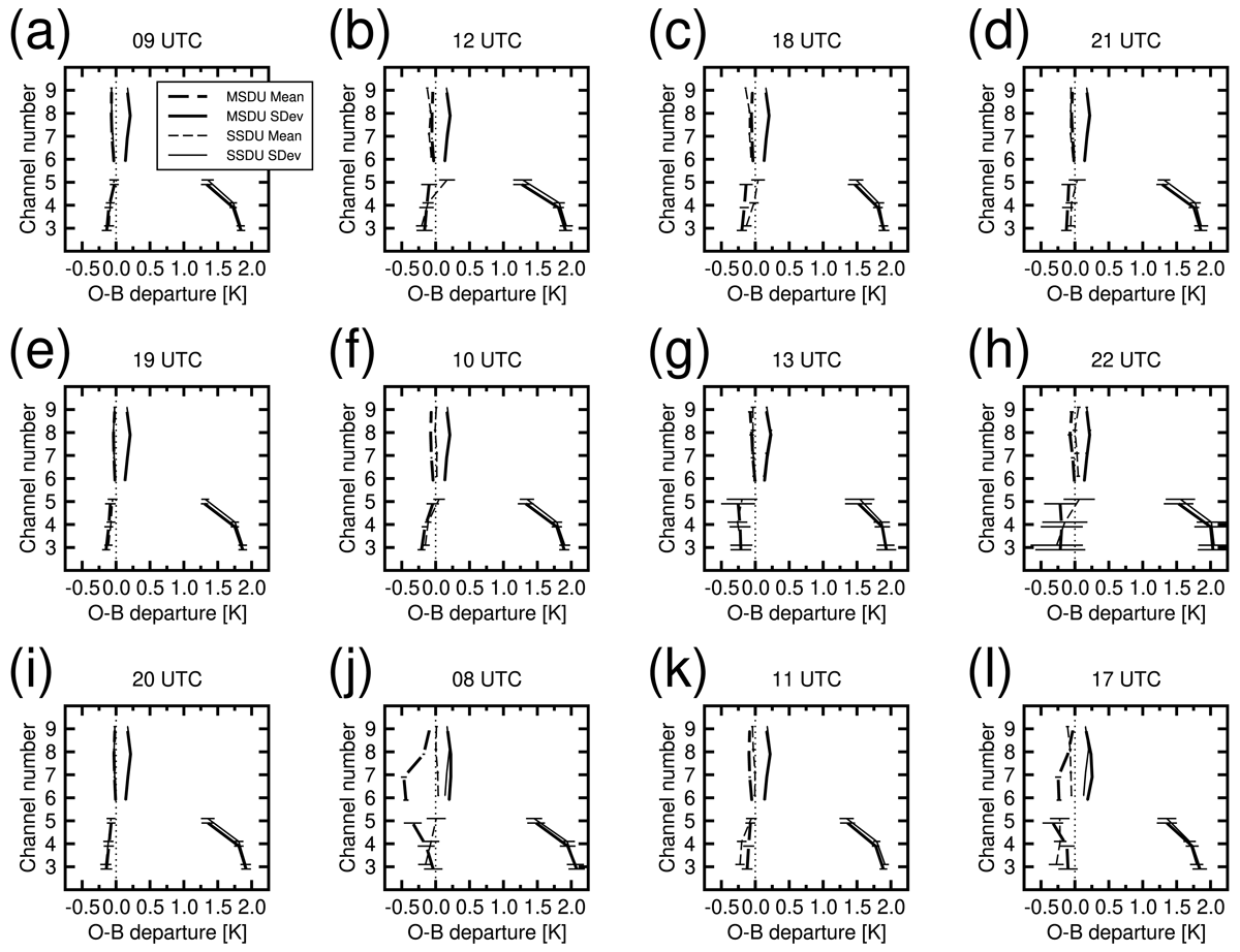
Figure 8
Observation minus background (O-B) departure statistics in the actively-assimilated microwave sounder channels of Metop-C. Channel indices go from 3 to 5 in MHS and from 6 to 9 in AMSU-A. Lines are as in Figure 7.
In the case of NOAA-20 (Figure 7), the temperature-sounding channels of ATMS are at indices 7–10 along the y-axis, while the humidity-sounding channels are at indices 19–22. In comparison with the MSDU scheme (thick lines), the SSDU scheme (thin lines) provides improved data fit at 00, 09, 04, 10, 05, and 08 UTC analysis hours. At all these hours, either mean or standard deviation (or both) of O-B are on average closer to zero in the SSDU test run than in the MSDU control run. The difference is in most cases significant at 95% confidence level. There is opposite behaviour, i.e., the data fit is degraded in the SSDU test run, at 12 and 13 UTC. At other analysis times, there either is very little difference between the two, or the superiority is controversial.
In the case of Metop-C (Figure 8), the temperature-sounding channels of AMSU-A are at indices 6–9 on the y-axis, while the humidity-sounding channels of MHS correspond to indices 3–5. The SSDU scheme indicates superior performance in fitting the data at 18, 21, 10, 22, and 08 UTC. At no analysis time does the SSDU perform worse than MSDU overall, but there is a notable degradation in the fit to humidity-sounding channels at 11 and 17 UTC.
On balance, in terms of the data fit, the SSDU test runs outperform the MSDU controls at more analysis hours than vice versa. Judging against the frequency distributions as a function of scan position (shown in Figure 5), there is a feel that the SSDU scheme performs better at times when the data coverage is strongly skewed towards either end of the range of scan positions. At times when the data coverage is more evenly distributed across the scan positions, the MSDU scheme is robust and there is no added benefit from switching to the SSDU scheme.
4.2.3 The impact on the background fit to independent data types
The next step is to evaluate the performance of the SSDU scheme in terms of short-range forecast accuracy. The common approach is to compute statistical measures of O-B departure in independent observation types and compare with the same score computed from the control run. Such a comparison is shown in Figure 9 for the case of a combination of radiosonde and aircraft measurement data. In this experiment and also in HARMONIE-AROME systems in general, these conventional observation types are handled without applying any bias correction. The statistic shown is the standard deviation of O-B departure in the test runs, but the scores are normalized with the equivalent score in the control runs. The bars indicate the 95% confidence intervals. The figure shows only a few examples of a statistically significant signal. The vector wind score shows up to 0.5% reduction, i.e., a positive impact, in the test run at S0 hours (panel (a)). The experiment runs at the S1 and S2 hours do not show a similar feature (panels (b) and (c)). The temperature scores higher than the 1000 hPa pressure level (panels (d)–(f)) are exclusively within the confidence intervals. At the 1000 hPa level, all three test runs consistently indicate a small negative impact, which is a potential source of concern. The experiments make only little use of low-peaking channels that could be directly attributed to this signal. There is a possible connection with the lowest-peaking channels of MHS and MWHS-2, since these channels are assimilated both over sea and over low-orography land areas south of the latitude 55°N. The significance of this possibility remains a topic of further investigation. The scores computed from humidity data (panels (g)–(i)) are not conclusive.
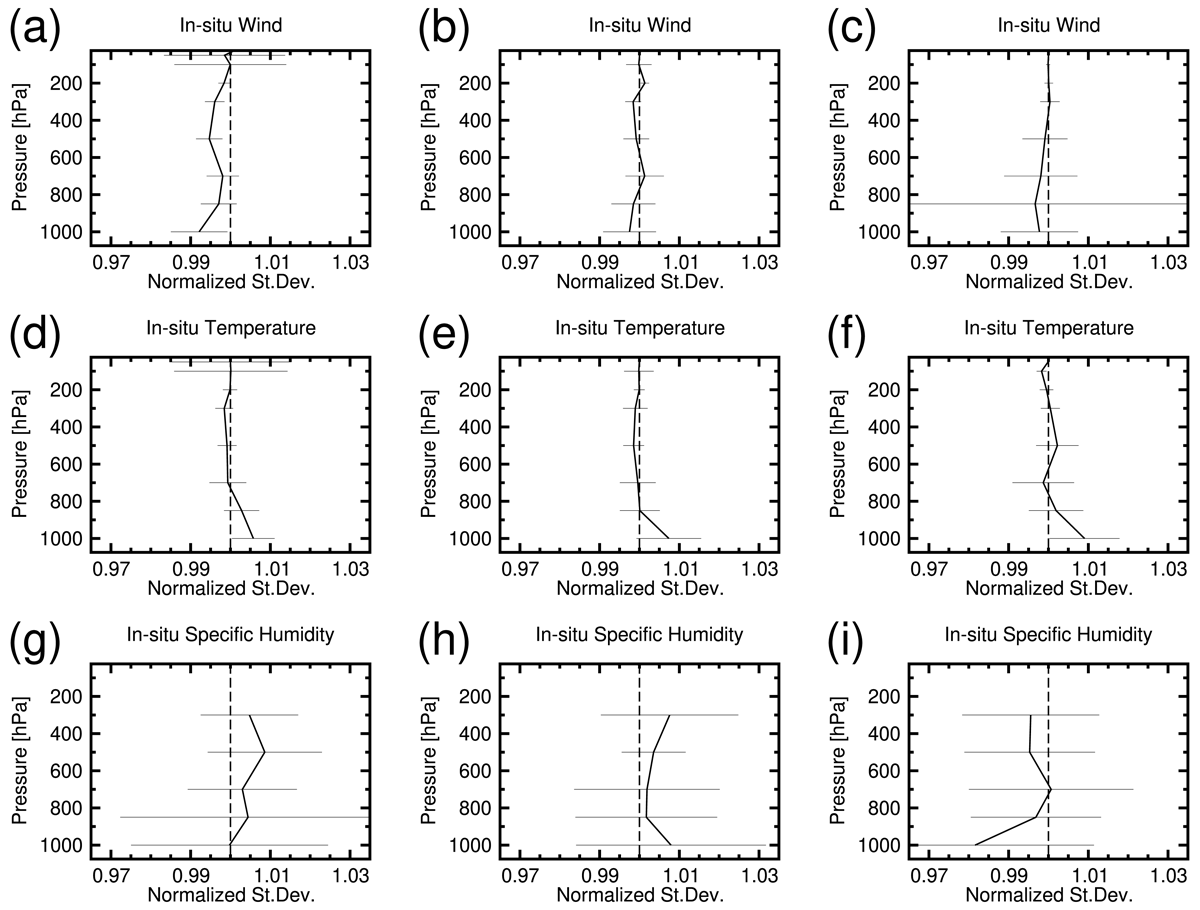
Figure 9
Short-range forecast impact of switching from MSDU to SSDU. The O-B data fit is shown in independent conventional measurements based on radiosondes and aircraft reports. The score is the control-normalized standard deviation of the O-B departure such that x-axis values less than one indicate a positive impact. The bars show the confidence intervals at 95% statistical significance level. (a)–(c) vector wind, (d)–(f) temperature, and (g)–(i) specific humidity. Panels (a), (d), and (g) are from the experiment run at S0 hours, panels (b), (e), and (h) at S1 hours, and panels (c), (f), and (i) at S2 hours.
4.2.4 The impact on forecast system performance
The final step of the performance evaluation assesses the impact on forecast scores at lead times relevant in limited-area NWP. Verification scores computed against observations taken at synoptic ground stations are shown in Figure 10. The figure shows root-mean-square of forecast error in the test runs at the S0 (panels (a), (d), and (g)), S1 (panels (b), (e), and (h)), and S2 (panels (c), (f), and (i)) hours. In each case, the score is normalized by its counterpart in the respective control run, such that negative values along the y-axis are indicative of a positive impact in the test runs. Again, the bars indicate the confidence intervals at the 95% significance level. Also in this verification there are only a few indications of statistically significant impact. The most notable impact is in the verification of mean sea level pressure in the test run at S2 hours (panel (c)). The statistically significant positive impact there reaches out to 12 hour forecast range, but no further. There are weak suggestions of isolated significant impacts (some positive, some negative) also in panels (b), (d), (f), and (h). Overall, we must conclude that the forecast verification provides no solid evidence of either positive or negative impact.
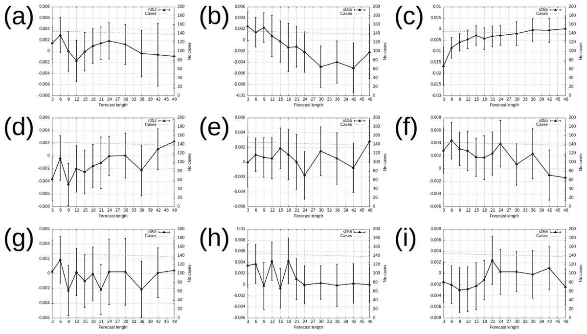
Figure 10
Forecast verification of switching from MSDU to SSDU. The scores are computed against verifying observations taken at synoptic ground stations. The score is the control-normalized root-mean-square of forecast error and positive impact manifests itself by negative values on the y-axis. The bars indicate the confidence intervals at 95% statistical significance level. (a)–(c) mean sea level pressure, (d)–(f) temperature, and (g)–(i) specific humidity. Panels (a), (d), and (g) are from the experiment run at S0 hours, panels (b), (e), and (h) at S1 hours, and panels (c), (f), and (i) at S2 hours.
5 Conclusions and future prospects
We have presented an evaluation of a specific variant (SSDU) of the VarBC algorithm tailored for the use in convective-scale limited-area NWP systems. The SSDU variant is intended as an alternative to the MSDU variant that is part of most operational implementations within the ACCORD consortium. The specific feature of SSDU is to allow only one daily update to the VarBC coefficients and otherwise keep them fixed during the analysis. However, the hour of the daily update is chosen separately for each polar orbiter. The underlying assumption is that doing the one daily update at an appropriate time is sufficient to ensure validity of VarBC coefficients at all analysis times.
The proposed setup is evaluated in the context of the operational convective-scale 3D-Var data assimilation system of the MetCoOp group. Switching from MSDU to SSDU is found to provide no statistically significant impact on forecast quality, although there are relatively minor improvements in the radiance data fit against the NWP model background. Overall the results are sufficiently encouraging for operational implementation in MetCoOp NWP suites.
The SSDU variant may allow to proceed towards assimilating polar-orbiting satellite data at all analysis times in limited-area NWP systems. The MSDU variant is unable to maintain robust VarBC coefficient information at those analysis hours when data coverage inside the computing domain tends to be poor. Such data is currently blacklisted from entering the assimilation. There is an associated excess burden via the need to reconsider the blacklisting hours from time to time for each satellite. From the point of view of technical maintenance, it would be desirable to remove the need for such blacklisting. No major meteorological impact is expected from such development though, since the number of additional data in the assimilation would be low.
There is a possibility to further improve the robustness of the bias correction through introducing automated recognition of sufficient representativeness in the sampling of predictors. The proposed SSDU variant involves a manual step to identify the analysis hour of the daily update for each satellite. Particularly with satellites in drifting orbits, the hour of the update will need to be revisited every now and then. The automated approach would avoid this manual work. Furthermore, an automated scheme would open up a possibility to assimilate radiance data from satellites in non-sun-synchronous orbits.
Data Accessibility Statement
Analysis-time- and experiment-run-specific statistical data that is used in the production of the figures is available for download at https://drive.google.com/file/d/1SOTUYikBrK4TKyxZLtNm_seckIHh-ead.
Acknowledgements
The author thanks Magnus Lindskog (Swedish Meteorological and Hydrological Institute) and Roger Randriamampianina (Norwegian Meteorological Institute) for general support and numerous practical suggestions on setting the SSDU scheme up in the HARMONIE-AROME reference system. He also acknowledges ECMWF for providing the HPC resources that were used in this work. Finally, he wishes to express his gratitude to an anonymous reviewer for providing constructive feedback and concrete suggestions to improve the manuscript.
Competing interests
The author has no competing interests to declare.