
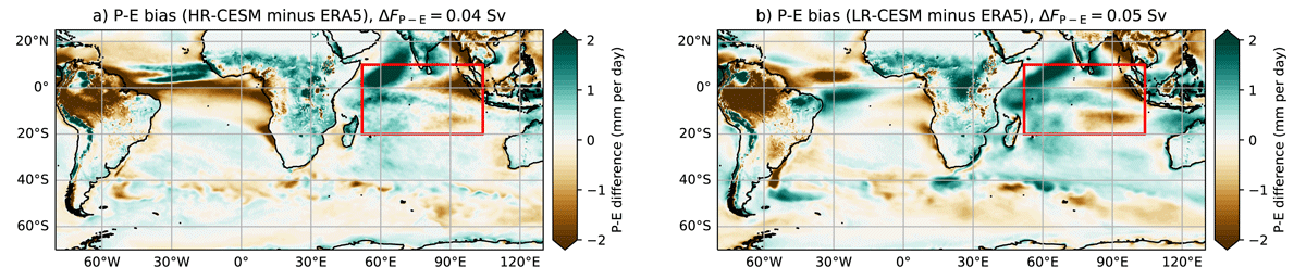
Figure 1
The present-day (1994–2020) P-E bias (w.r.t. ERA5) for the (a): HR-CESM and (b): LR-CESM. The spatially-averaged P-E biases over the red-outlined region are 0.04 Sv and 0.05 Sv, respectively.
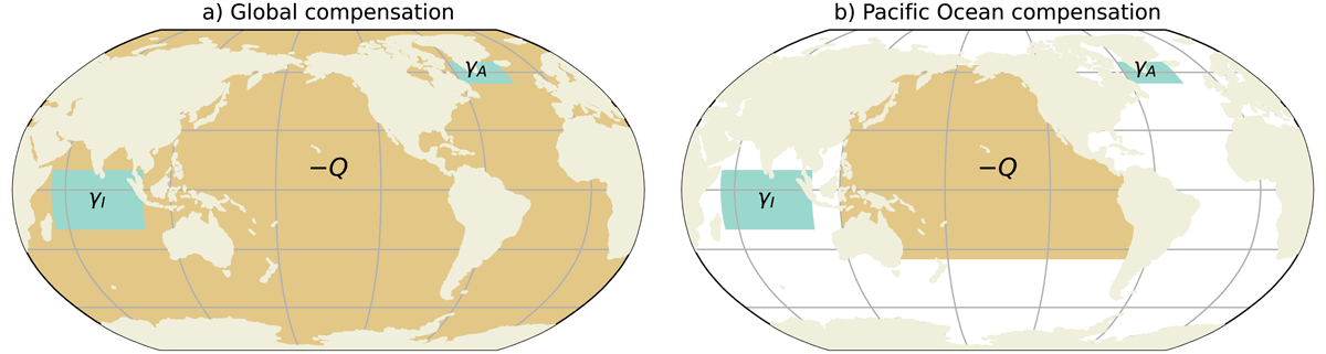
Figure 2
Areas where freshwater flux anomalies are applied with their strengths γA and γI; also the global compensation region (a) and the Pacific region (b) is shown.
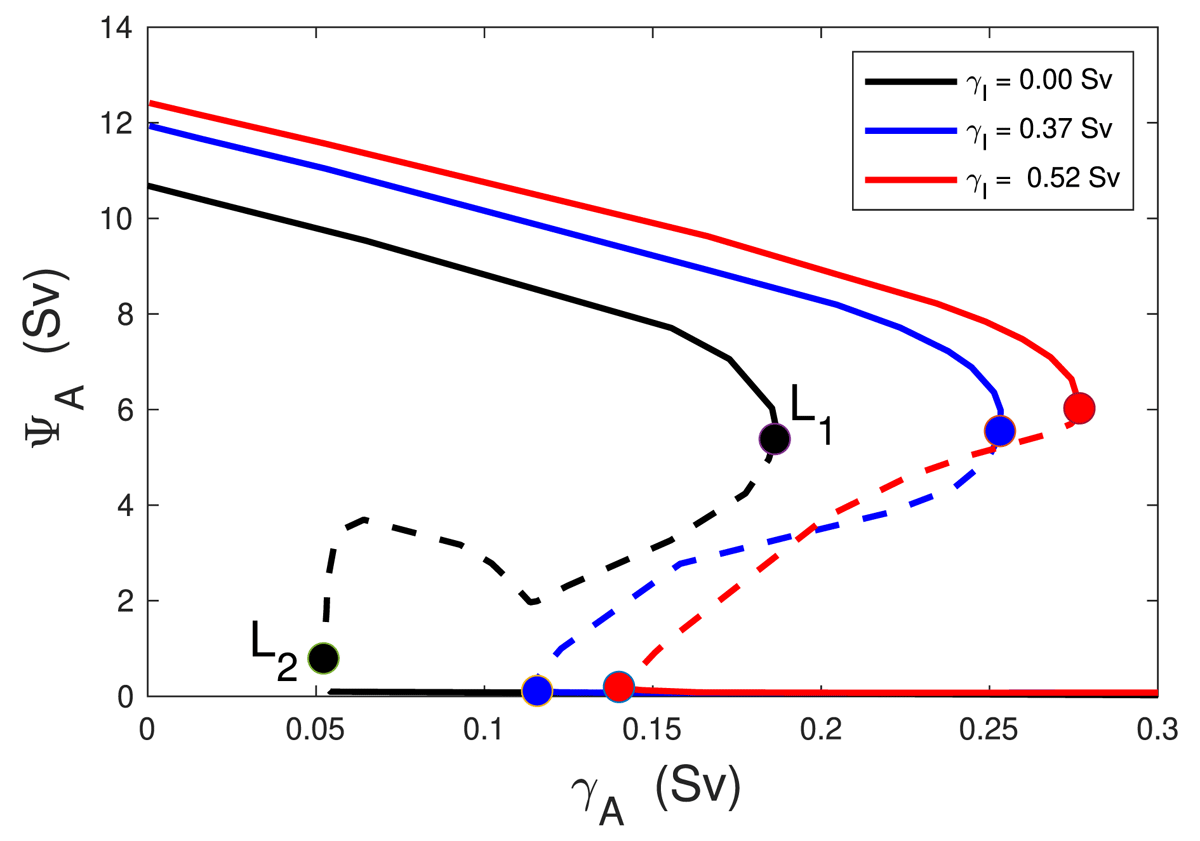
Figure 3
Bifurcation diagrams for the case of global compensation where the maximum strength of the AMOC below 1000 m (ΨA) is plotted versus the strength of the anomalous freshwater forcing γA for different values of γI. Solid (dashed) curves indicate stable (unstable) branches. The dots indicate the saddle-node bifurcations.
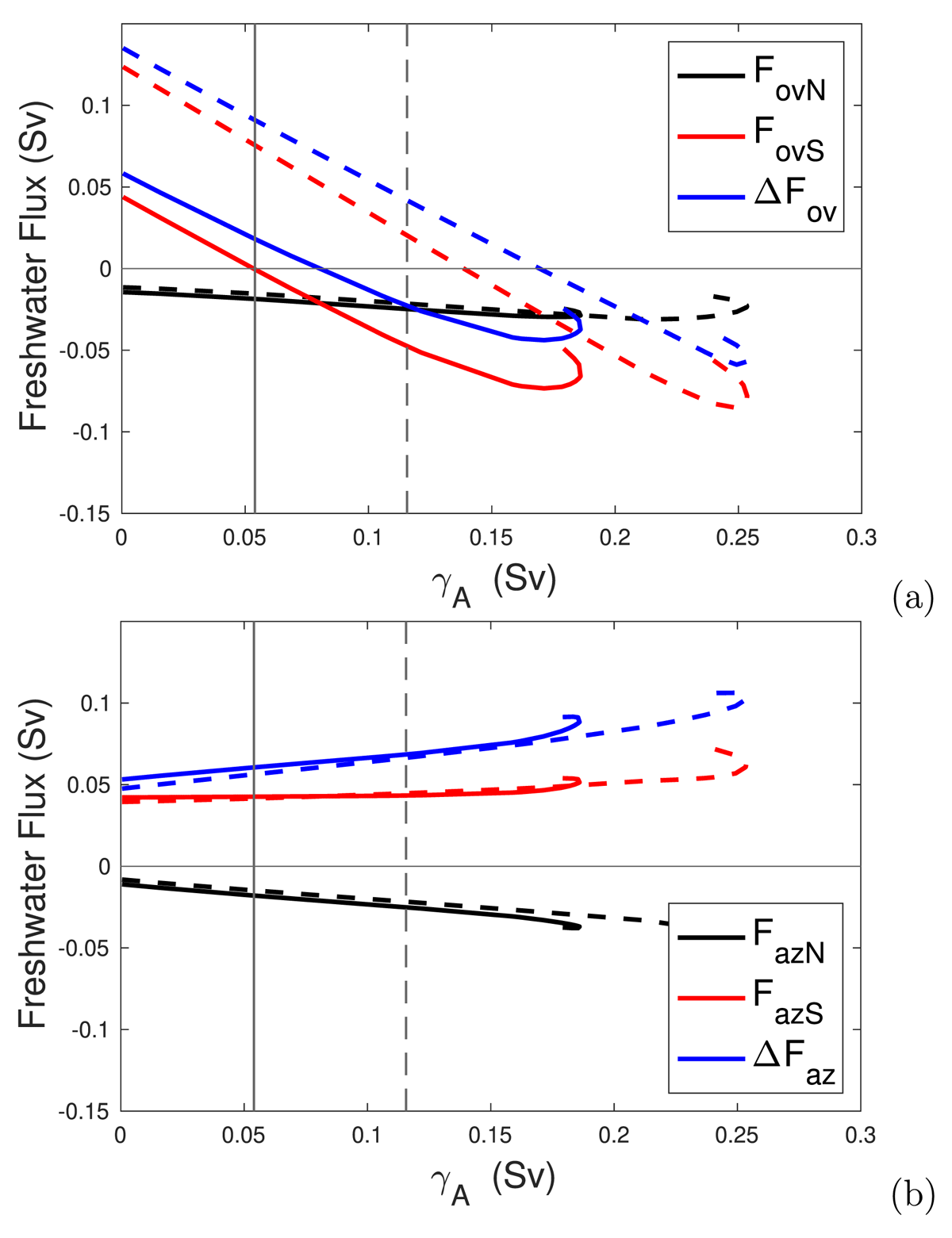
Figure 4
Global compensation case. (a) Values of the AMOC induced freshwater transport at the southern boundary (35°S) of the Atlantic (FovS), the northern boundary (60°N) of the Atlantic (FovN), and their difference ΔFov. (b) Same as (a) but for the azonal transport (FazS, FazN and ΔFaz). The vertical thin lines indicate the saddle-node bifurcation L2. The solid curves are for γI = 0, corresponding to the black curve in Figure 3. The dashed curves are for γI = 0.37 Sv, corresponding to the blue curve in Figure 3.
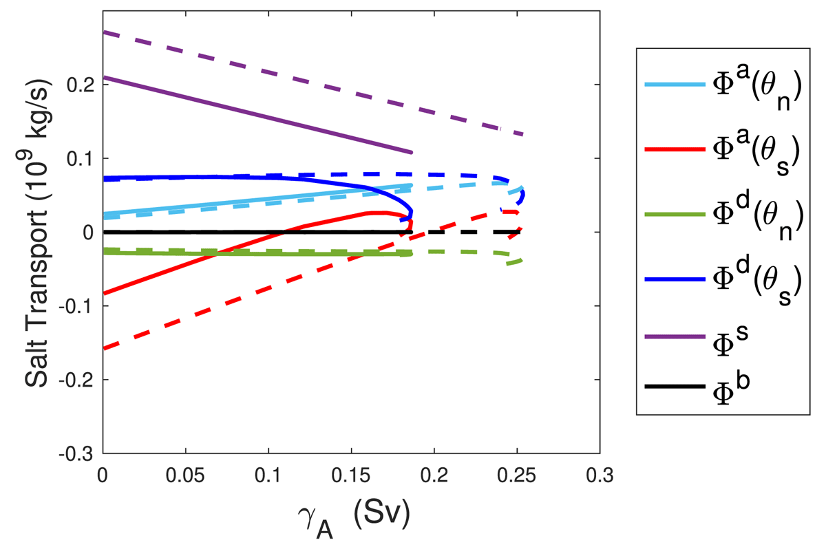
Figure 5
Global compensation case. Terms in the integrated salt balance over the Atlantic basin over the upper branches in Figure 3 (up to ), with expressions of the terms as indicated in equation (9) and equation (10) for θn = 60°N and θs = 35°S. The solid curves are for the case γI = 0 and the dashed ones for γI = 0.37 Sv.
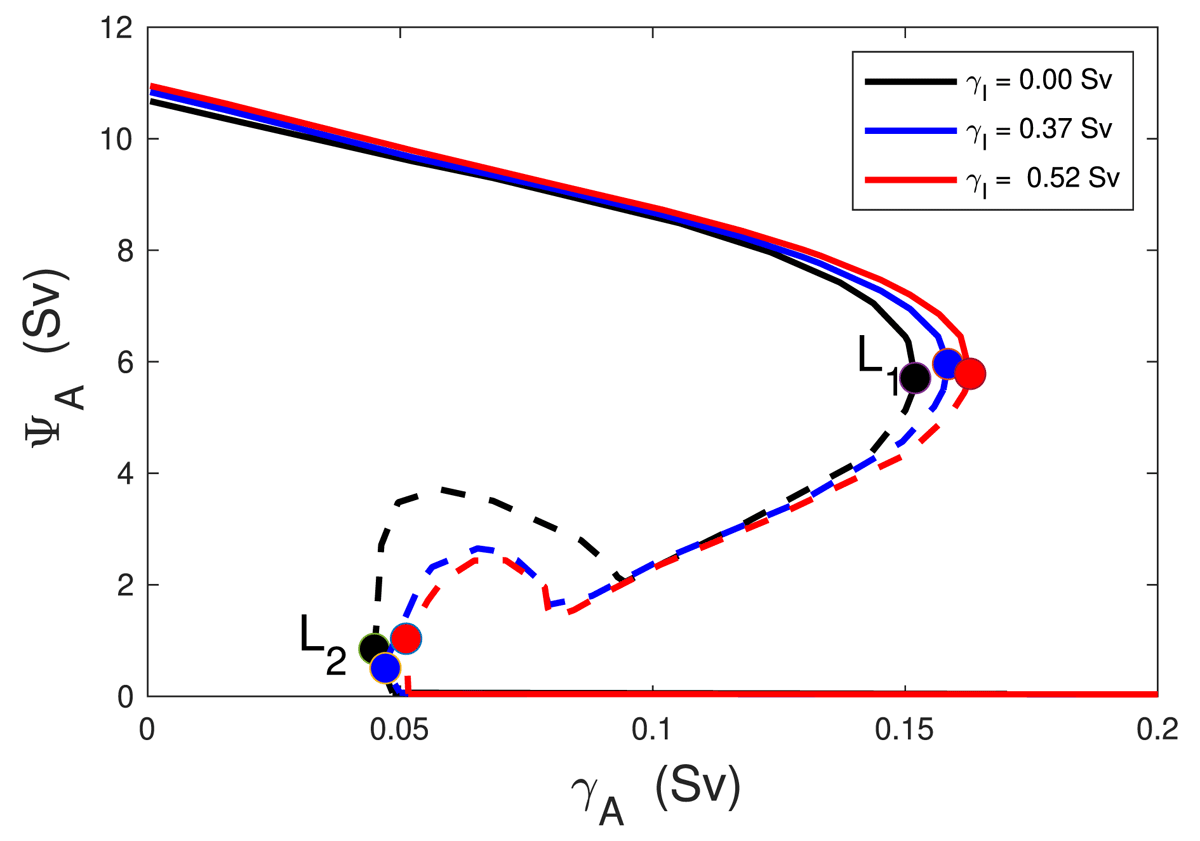
Figure 6
Bifurcation diagram for the case of Pacific compensation where the maximum strength of the AMOC below 1000 m (ΨA) is plotted versus the strength of the anomalous Atlantic freshwater forcing γA for different values of γI. The dots indicate the saddle-node bifurcations.
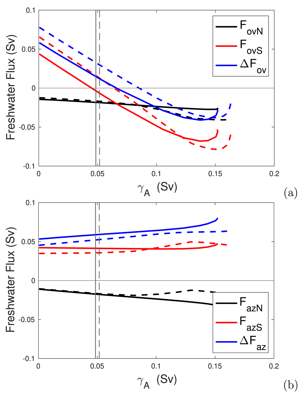
Figure 7
Pacific compensation case. (a) Values of the AMOC induced freshwater transport at the southern boundary (35°S) of the Atlantic (FovS), the northern boundary (60°N) of the Atlantic (FovN), and their difference (ΔFov). (b) Same as (a) but for the azonal transport (FazS, FazN and ΔFaz). The vertical thin lines indicate the saddle-node bifurcation L2. The solid curves are for γI = 0, corresponding to the black curve in Figure 6. The dashed curves are for γI = 0.52 Sv, corresponding to the red curves in Figure 6.
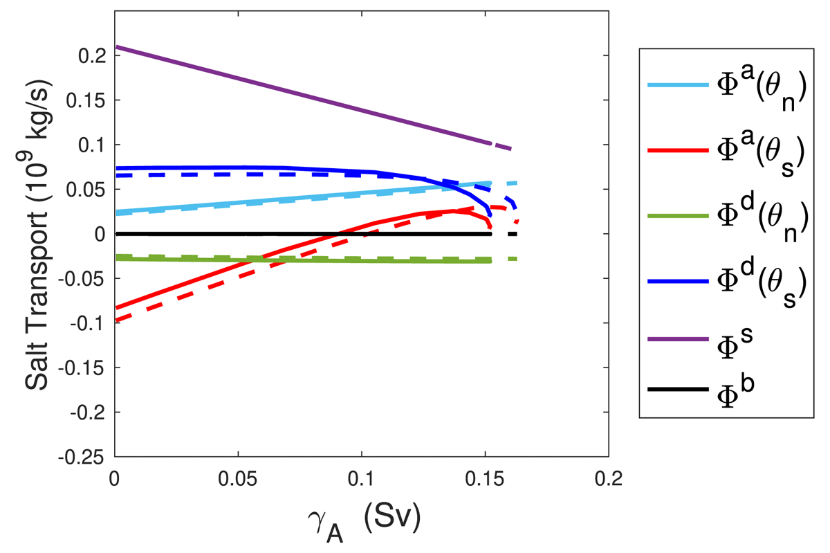
Figure 8
Pacific compensation case. Terms in the integrated salt balance over the Atlantic basin over the upper branch in Figure 6, with expressions of the terms as indicated in the main text. The solid curves are for the case γI = 0 and the dashed ones for γI = 0.52 Sv.