
1 Introduction
A tropical cyclone (TC) is a low-pressure eddy that occurs over the surface of tropical or subtropical oceans. TCs occur in the Northern Hemisphere more than in the Southern Hemisphere, and two thirds of the TCs that occur globally each year come from the Northern Hemisphere (Valorie Crooks, 2021). The life cycle of TCs can be roughly divided into four stages: generation, development, maturity and dissipation. In general, TCs generated in the Western Pacific Ocean are called typhoons, while TCs in the Atlantic and Northeast Pacific Ocean are called hurricanes, and tropical cyclones in the Indian Ocean.
Numerous studies on cyclone-induced marine changes have been published in recent decades. The sea surface temperature (SST) is the key factor in cyclone-ocean energy exchange. SST usually descends after TCs pass due to cold water lifted to the sea surface (Ji et al., 2021), which will affect the intensity of TCs. When SST cooling exceeds 2.5°C, it is considered to be unfavorable to TC strengthening and even weakening (Schade et al., 1999), which will change the trajectory and strength of TCs (Zhang et al., 2021). TCs often trigger phytoplankton blooms, which contribute to improving local primary productivity. The entrainment and upwelling caused by ocean cyclonic eddies can provide a favorable environment for the sea surface phytoplankton bloom (Ji et al., 2021). For example, the mean concentration of Chl-a increased from 0.2 mg•m–3 to 0.53 mg•m–3 after the passage of Hurricane Katrina in the Gulf of Mexico in 2005, peaking at 2.69 mg•m–3 for four days after the passage of Katrina (Gierach and Subrahmanyam, 2008). During Typhoon Kai-tak’s brief stay in the South China Sea in 2000, the sea surface concentration of Chl-a increased by an average of 30 times (Lin et al., 2003). Other examples of this phenomenon include Typhoon Damrey in 2005 (Zheng and Tang, 2007) and Typhoon Nuri in 2008 (Zhao et al., 2009). Additionally, near-inertial internal waves have also been observed during and after the passage of TCs (Zheng et al., 2020), which will exert force and torque on cylindrical tendon legs (Lü et al., 2016). Strong typhoons can cause turbulent mixing, which can cause the sediment to resuspend and provide favorable conditions for phytoplankton blooms (Li et al., 2021).
The Northern Indian Ocean is subdivided by the Bay of Bengal and the Arabian Sea. TCs are generated mainly in the Bay of Bengal, which is 5-6 times more prevalent than that in the Arabian Sea (Lu et al., 2020). The upper ocean is well stratified in the Bay of Bengal, where the perennial barrier layer lies between the mixed layer and the isothermal layer (He et al., 2017; Kuttippurath et al., 2021). This barrier layer can restrain the exchange of substances between the ocean subsurface layer and the surface layer (Thadathil et al., 2007; Balaguru et al., 2012). Compared with other regions, the TCs in the Bay of Bengal receive more and more attention because of their shallow depth, low-lying coastal terrain and funnel-shaped coastline features (Roy Chowdhury et al., 2021), strong winds, heavy rain, storm surge and phytoplankton blooms during and after the passage of TCs (Lu et al., 2020). In the Bay of Bengal, phytoplankton blooms triggered by TCs Thane and Phailin were influenced by physical processes in the upper oceans rather than the intensity of the TCs (P.J et al., 2017). The mechanisms of phytoplankton blooms induced by the TCs Fanoos, Nisha, and Nilam are also studied from the perspective of Ekman pumping velocity and translational speed of TCs (Sunanda et al., 2018).The above studies on the factors of Marine biological response caused by cyclones are mostly considered from the aspects of cyclone characteristics (intensity, residence time) and Marine environmental conditions (SSH, SST). However, there has been little discussion of the effects on phytoplankton blooms during the transit of TCs from the perspective of upper cyclonic eddies and submarine anticyclonic eddies. Interestingly, the sea surface response from cyclones usually calmed down after a week or a few weeks (Zhang et al., 2021), but why did the chlorophyll concentration peak again after the passage of TC Hibaru in January 2005?
In this study, the phytoplankton blooms after the passage of TC Hibaru in January 2005 were studied with satellite observations, multisource reanalysis products and Argo float data. It was first observed that an ocean anticyclonic eddy in the subsurface moves westard under a surface cyclonic eddy in southeastern Sri Lanka, which triggered the second Chl-a bloom. the data and methods are presented in Section 2, physical and biochemical reactions are described in Section 3, possible mechanisms are discussed in Section 4, and the conclusion is summarized in Section 5.
2 Data and methods
2.1 Study area
In this study, we selected Box A (3.5° N-6° N, 83.5° E-88.5° E) along the TC path (Figure 1). TC Hibaru formed over southeastern Sri Lanka on January 11 and was upgraded to a cyclonic storm by the India Meteorological Department (IMD) on January 15. It drifted southward and slowly weakened before dissipating on January 17.
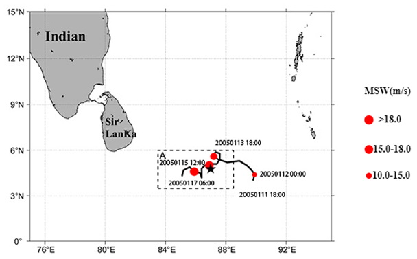
Figure 1
The tracks of TC Hibaru and the TC centers are shown by black lines and red dots, respectively. The black dashed line frames the study area. Box A: 3.5° N-6° N, 83.5° E-88.5° E.The position of the Argo is indicated by the black star.
2.2 Data
The data source of the best path of the typhoon was cyclone data released by the United States Guam Joint Typhoon Warning Center (JTWC).These datasets contain additional information such as the center position of the typhoon, maximum wind speed, minimum pressure and intensity level (https://www.metoc.navy.mil/jtwc/jtwc.html).
The SST data are derived from remote sensing systems. It provides SST products for studying the SST variation. The product had a spatial resolution of 0.25 degrees and is the result of the fusion of multiple microwave and infrared satellite sensors through optimal interpolation (http://www.remss.com/).
The calculation data of the monthly average precipitation in the research area is sourced from the 3B42 product provided by the Tropical Rainfall Measuring Mission (TRMM) project, with a temporal accuracy of 3 hours and a spatial accuracy of 0.25 degrees (https://daac.gsfc.nasa.gov/).
The near-real-time daily sea surface height (SSH), high resolutions (0.083° × 0.083°) sea current velocity and Chl-a data were obtained from the Global Ocean Physics Reanalysis product supplied by the Copernicus Marine Environment Monitoring Service (CMEMS, http://marine.copernicus.eu/). In scientific research, this dataset is widely used (Xia et al., 2022; Tan et al., 2022).
The Indian Argo project provides temperature and salinity data within 200 m below the sea surface (https://dataselection.euro-argo.eu/). In Figure 1, red pentagram shape is used to represent the buoy position.The Argo platform number used in this study is 2900352.
2.3 Methods
2.3.1 Vorticity
The calculation formula for the curl of the current vector (u,v) is as follows (Xia et al., 2022).
where u and v denote the velocity components along the x and y directions, respectively.
2.3.2 Barrier Layer Thickness
The density, mixing layer depth (MLD), isothermal layer depth (ILD) and barrier layer thickness (BLT)were calculated in the study area (He et al., 2020). MLD was defined as the increase in potential density by Δσθ when SST decreases by 0.5(ΔT = –0.5°C), which is equal to the depth of the increase in potential density.
where T0, S0 and P0 denote the temperature, salinity and pressure values of the sea surface, respectively. When the temperature is 0.5°C less than the sea surface temperature, the depth (D) at this time is called the isothermal layer depth (ILD).
BLT is defined as the difference between ILD and MLD.
3 Results
3.1 Description of Hibaru
On January 10, a convective zone was formed over the southeastern Sri Lanka with a low wind shear. In the following days, it became a deep depression on January 14 and intensified into a cyclonic storm the next day, with wind speed of 65 km per hour. The TC then drifted south and slowly weakened. On January 17, Hibaru degenerated into a remnant (Table 1).
Table 1
Position, time and MWS (maximum wind speed) of TC Hibaru.
| LATITUDE (°N) | LONGITUDE (°E) | TIME | MWS (M•S–1) |
|---|---|---|---|
| 4.0 | 89.8 | 2005/01/11/18 | 10.289 |
| 4.4 | 89.9 | 2005/01/12/00 | 10.289 |
| 4.7 | 89.7 | 2005/01/12/06 | 10.289 |
| 5.0 | 89.4 | 2005/01/12/12 | 10.289 |
| 5.3 | 88.9 | 2005/01/12/18 | 10.289 |
| 5.2 | 88.1 | 2005/01/13/00 | 12.861 |
| 5.4 | 87.5 | 2005/01/13/06 | 15.433 |
| 5.6 | 87.2 | 2005/01/13/12 | 15.433 |
| 5.9 | 87.3 | 2005/01/13/18 | 15.433 |
| 5.8 | 87.6 | 2005/01/14/00 | 15.433 |
| 5.4 | 87.6 | 2005/01/14/06 | 15.433 |
| 5.1 | 89.6 | 2005/01/14/12 | 18.005 |
| 5.1 | 87.4 | 2005/01/14/18 | 18.005 |
| 5.0 | 87.1 | 2005/01/15/00 | 18.005 |
| 5.0 | 86.9 | 2005/01/15/06 | 18.005 |
| 4.8 | 86.6 | 2005/01/15/12 | 18.005 |
| 4.5 | 86.4 | 2005/01/15/18 | 18.005 |
| 4.2 | 86.4 | 2005/01/16/00 | 18.005 |
| 4.5 | 86.3 | 2005/01/16/06 | 18.005 |
| 4.6 | 85.9 | 2005/01/16/12 | 18.005 |
| 4.9 | 85.6 | 2005/01/16/18 | 15.433 |
| 4.7 | 85.2 | 2005/01/17/00 | 12.861 |
| 4.3 | 85.1 | 2005/01/17/06 | 10.289 |
3.2 Chl-a
The sea surface Chl-a distribution and surface current during (January 14) and after (January 20) the passage of the TC are shown in Figure 2. As seen in Figure 2, the surface Chl-a concentration increased significantly after the passage of TC. Two peak values of phytoplankton blooms with the surface cyclonic eddy were observed from January 19 to 20 and January 27 to 28, where the maximum Chl-a concentrations were 0.235 mg•m–3 and 0.124 mg•m–3, respectively (Figure 3). It is noteworthy that the first (second) peak occurred on the second (tenth) day after the passage of the TC. There is no surface phytoplankton blooms during the passage of the TC, which may be because cloud cover hinders light and prevents photosynthesis (Roy Chowdhury et al., 2021). When the TC leaves, the clouds dissipate, sunlight reaches the sea surface and photosynthesis takes place, so that changes in the surface Chl-a can be better captured (Gierach and Subrahmanyam, 2008). The vertical distribution of Chl-a concentrations in Box A from January 1 to 30 is shown in Figure 4. It was obvious that the subsurface Chl-a was uplifted to the sea surface with upwelling during the periods of the two phytoplankton blooms.
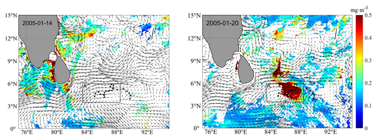
Figure 2
Surface Chl-a distribution on January 14 (a) and January 20 (b). Black arrows indicate sea surface currents.
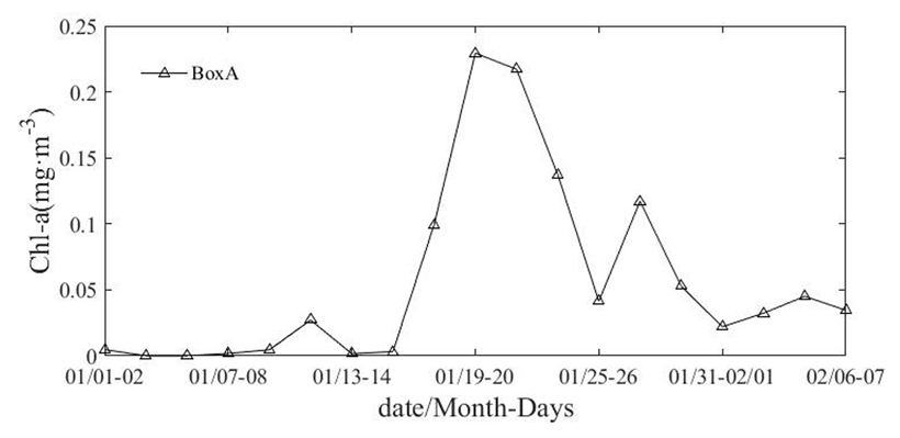
Figure 3
The change curve of two-day averaged Chl-a concentration in Box A from January 1 to February 7.
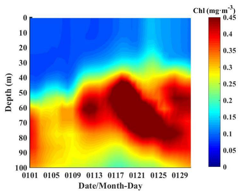
Figure 4
The vertical distribution of Chl-a concentration in Box A from January 1 to 30.
Horizontal advection may also cause changes in chlorophyll concentrations (Xu et al., 2021). Figure 5 shows the Chl-a fluxes around Box A from January 1 to 29. The north-south (east-west) Chl-a concentration is multiplied by V (U) to calculate the north-south (east-west) Chl-a fluxs of Box A. On the south and west sides, positive fluxes are inflows and negative ones are outflows. On the north and east sides, positive fluxes are outflows and negative ones are inflows. It can be found that Chl-a in Box A is mainly transported horizontally from the eastern and southern sides (Figure 5), which are also related to the direction of the sea current (Figure 2).
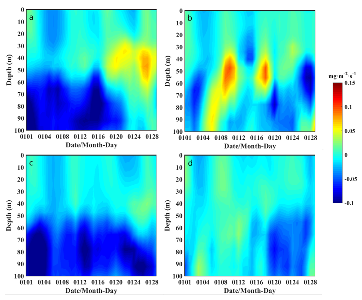
Figure 5
Time series of Chl-a fluxes in the eastern (a), southern (b), western (c) and northern (d) sides of Box A from January 1 to 28.
3.3 SSH, SST, Current and Barrier Layer
Generally, the production of Chl-a at the sea surface depends on the amount of nutrients brought from the ocean floor by upwelling (Price, 1981) and subsurface ocean processes such as Ekman upwelling (Sunanda et al., 2018). As shown in Figure 6, a cyclonic ocean eddy moved slowly from east to the west into the study area from January 11 to 19 (Figure 6 a–d). The minimum SSH at the cyclonic eddy center was 0.18 m due to the surface current divergence. The current at a depth of 75 m and the surface current from January 25 to 26 are shown in Figure 6e–h. There was an anticyclonic ocean eddy slowly moving into Box A, while the sea surface is a cyclonic eddy at this time, which may be one of the important factors leading to strong vertical mixing, thus producing the second Chl-a bloom. The possible driving mechanism will be analyzed in the next section.
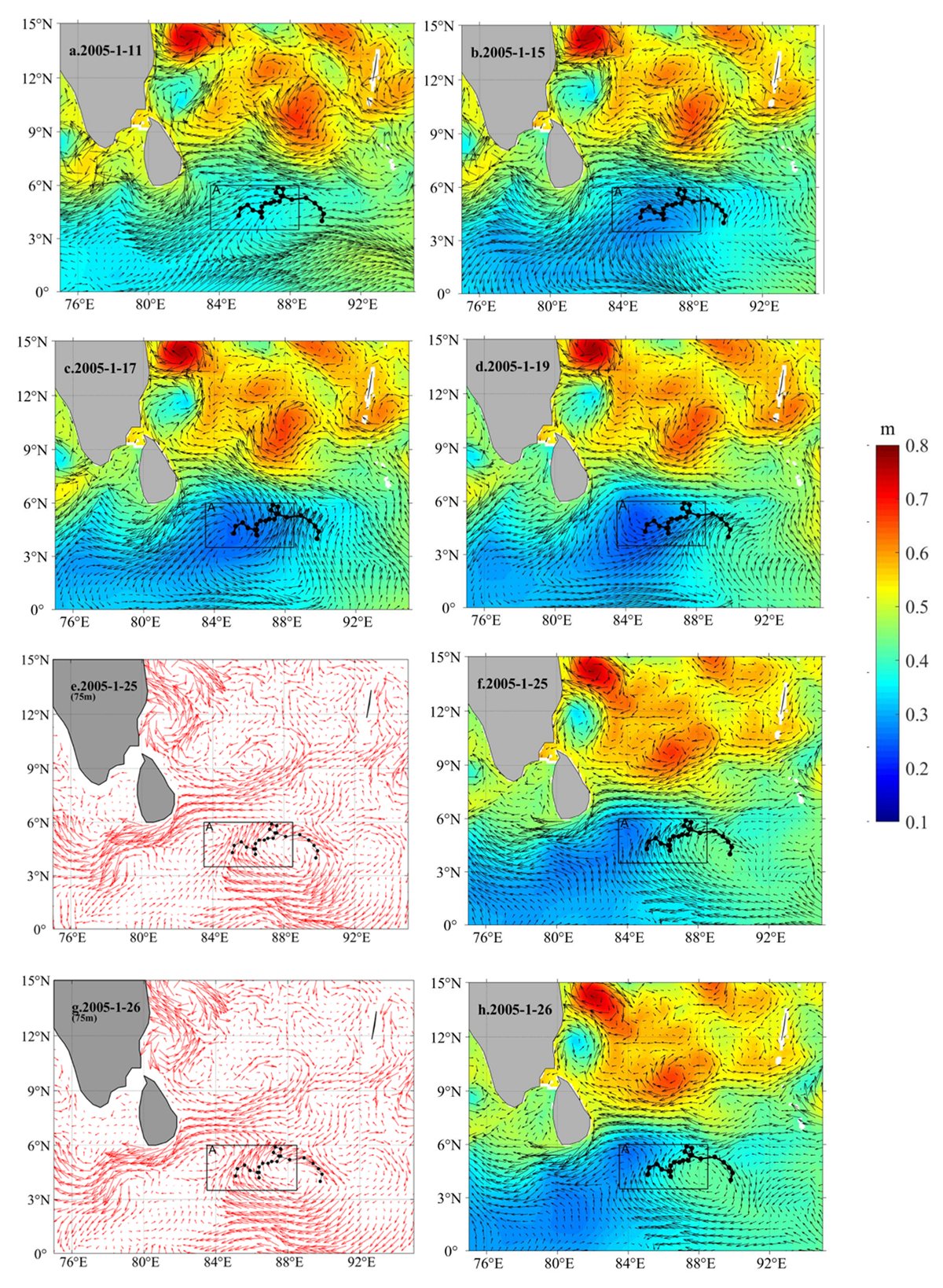
Figure 6
Sea surface height (SSH) and current on January 11, 15, 17 and 19 (a, b, c, d). The sea current is represented by a black arrow, and the color bar represents the SSH. On January 25 and 26, the currents at a depth of 75 m are represented by red arrows (e, g).The black arrows (f, h) shows the direction of the surface current.
At the center of the cyclonic eddy, there is a cold updraft that enhances sea surface cooling, while there is a warm downdraft at the center of the anticyclone that hinders sea surface cooling (Gierach and Subrahmanyam, 2008; Zhang et al., 2021). Figure 7 illustrates the vertical distribution of temperature over time from January 1 to 30 in Box A. Between January 5 and 8, prior to the passage of Hibaru, the SST in the research area exceeded 28°C. During the Hibaru transit period, a significant surface cooling occurred with a decrease of 2 °C, caused by upwelling around the cyclonic eddy center.
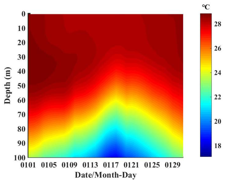
Figure 7
The vertical distribution of temperature over time in Box A from January 1 to 30 .
Nitrate nitrogen concentration was linearly and negatively correlated with SST. The lower the temperature, the higher the nitrate content instead (Chen et al., 2006). This implies that a decrease in SST can reflect, to some extent, the vertical transport of nutrients from the deep sea. SST decreases are usually associated with high nutrient vertical supply (Siswanto et al., 2022). During the passage of TC Hibaru, SST decreased on 13 January (Figure 7), PAR increased over time (Figure 10).The trend of these two factors was so consistent over a period of time, followed by a large increase of two-day averaged Chl-a concentration (Figure 3). Generally, there is a lag between TC and phytoplankton blooms because of the time required to raise nutrient-adequate cold deep water to the surface via upwelling (Valorie Crooks, 2021), which drives the upper ocean to produce large amounts of biological production through photosynthesis (Narvekar et al., 2021) .
Additionally, there is usually a distinct barrier layer throughout the year in the Bay of Bengal (He et al., 2017; Kuttippurath et al., 2021). The depth difference between the mixed layer depth (MLD) and the isothermal layer depth (ILD) is calculated by Formula 7, which is the barrier layer thickness (BLT). Figure 8 shows the BLT calculated with argo data on January 14 and 29. The BLT was reduced from 19.9 m to 14.77 m. The ocean barrier layer can impede the vertical exchange between the mixed layer and the deep ocean and has a critical role in the study of ocean biochemistry and air-sea heat fluxes (Pothapakula et al., 2017). It can be found that the weakened BLT helps to the uplift of the deep sea Chl-a and nutrients to the sea surface through upwelling.
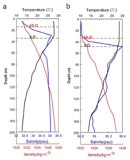
Figure 8
Barrier layer thickness calculated from Argo data in Box A on January 14 and 29.
3.4 Precipitation
TCs often bring strong winds and heavy rainfall (Balaguru et al., 2022). Figure 9 shows the spatially averaged precipitation for Box A from January 1 to 31. From January 11 to 17, the precipitation in Box A was almost zero and started to increase on January 18, reaching a maximum of 2.23 mm on January 21. Heavy rainfall can weaken TC-induced mixing, which in turn limits ocean surface cooling (Jourdain et al., 2013;Zhang et al., 2021). In this study, significant precipitation occurred for seven days after TC transit.
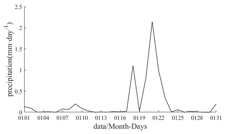
Figure 9
The spatially averaged precipitation for Box A from January 1 to 31.
3.5 Photosynthetically available radiation (PAR)
Curve of the spatial average PAR over time in Box A is shown in Figure 10. The PAR increased significantly after the passage of Hibaru. During the passage of Hibaru, the lowest PAR value occurred on January 13, which may be caused by atmospheric clouds. From January 19 to 22 and January 27 to 28, the bigger PAR means that an abundance of sunlight can enter the euphotic layer. Phytoplankton reproduction requires sunlight for photosynthesis, so PAR may be an important factor for the two phytoplankton blooms (Figure 3).
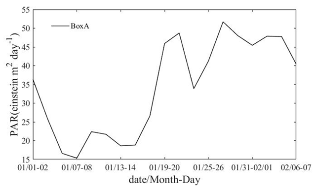
Figure 10
Curve of the spatial average PAR over time in Box A from Jan. 1 to Feb. 7.
4 Discussion
4.1 The role of stratification
Due to the strong reliance of mixing on the vertical density structure, ocean stratification plays an indispensable role in the study of TC responses. The mixed layer is a key factor affecting the surface Chl-a concentration (Chacko, 2019)during the movement of the TC.This is because the MLD is a key parameter in altering nutrient concentrations and light availability.The surface Chl-a concentration after the passage of TC often depends on the intensity of upwelling and mixing layer deepening (Chacko, 2019). The average nutrient line of most cyclones is almost shallow, and a deepened MLD more easily reaches the nutricline depth where nitrate concentrations are approximately equal to zero and begins to increase (Chacko, 2019), providing nutrient source for a later phytoplankton bloom.The buoyancy frequencies of Box A on January 9, 14, 19, 24, and 29 are shown in Figure 11. The buoyancy frequency was reduced from 0.027 s–1 to 0.023 s–1 (0.024s–1 to 0.017s–1) from January 9 to 14 (January 24 to 29), where the upper weakened stratification can lead to the accumulation of surface phytoplankton with upwelling for the two phytoplankton blooms after the passage of the TC. A similar situation was also observed in the other sea area in the Bay of Bengal by (P.J et al., 2017), where there were 2-fold and 7-fold increase in chlorophyll after the passage of Phailin and Thane, respectively.
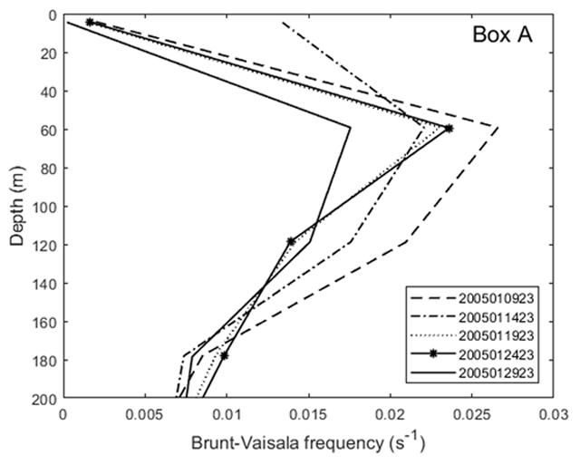
Figure 11
Vertical profile of the Argo buoyancy frequency of Box A, which includes six time points on January 9, 14, 19, 24 and 29.
Additionally,the variability of chlorophyll in the southwestern and western regions is more sensitive to nutrients from the deep sea than that in other regions of the Bay of Bengal (Siswanto et al., 2022). The absence of the barrier layer was conducive to the nutrient updraft caused by ocean cyclonic eddies and surface chlorophyll blooms (Balaguru et al., 2012;Li et al., 2022). In our study area, the BLT was reduced from 19.90 m to 14.77 m (Figure 8). The weakened barrier layer can create good conditions for upward nutrient transport.This suggests once again that the phytoplankton blooms are supported by nutrient entrainment rising into the euphotic layer.
4.2 Vorticity
The spatially averaged vorticity from January 1 to 31 in Box A is shown in Figure 12. Before the passage of Hibaru, there was a weak surface cyclonic eddy with vorticity less than 0.1 s–1 in Box A. During the Hibaru transit period, the cyclonic eddy was gradually strengthened, where the vorticity increased from 0.06 s–1 to 0.15 s–1. After the passage of Hibaru, the surface cyclonic vorticity reached a maximum of 0.18 s–1 on January 19, which can uplift nutrients and Chl-a from the deep sea to the upper sea. After January 21, the intensity of the surface cyclonic eddy gradually decreased, and the vorticity was 0.04 s–1 on January 26. However, on January 26, an anticyclonic eddy entered Box A in the subsurface layer ahead of the surface layer (Figure 6g–h), which appeared below a depth of 50 m. The subsurface anticyclonic eddy may contribute to the Chl-a and nutrient horizontal convergence (Figure 5), which can be uplifted to the sea surface through upwelling (Figures 4 and 7) by the surface cyclonic eddy (Figure 12) and weakened BLT (Figure 8).
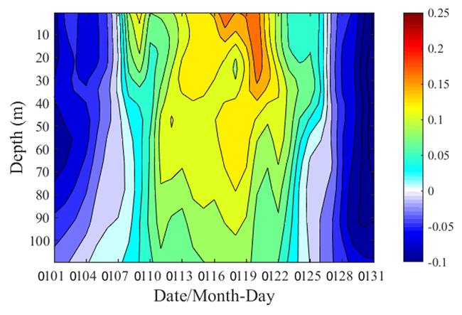
Figure 12
Time series of spatially averaged vorticity in Box A from January 1 to 31.
4.3 Mechanism Exploration
The dynamical mechanism of the first bloom is shown in Figure 13a. It may be caused by horizontal transport (Figure 5) and upwelling by the enhanced cyclonic eddy, which can uplift deeper nutrients and Chl-a to the surface layer (Figure 8). Photosynthesis with high PAR is carried out when nutrients are pumped up to the upper euphotic zone. Finally, the surface Chl-a concentration attains the maximum of 0.235 mg•m–3 from January 19 to 20.
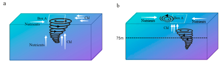
Figure 13
Schematic diagram of mechanisms for the first (a) and second (b) phytoplankton blooms in Box A.
The dynamic mechanism of the second Chl-a bloom from January 27 to 28 is shown in Figure 13b. As the surface cyclonic eddy moved westward after the passage of Hibaru, the anticyclonic eddy entered Box A on January 25 at the subsurface earlier than that at the sea surface. With the lower anticyclonic eddy, the subsurface chlorophyll horizontally converged by the subsurface anticyclonic eddy and was uplifted with upwelling by the weaker surface cyclonic eddy and weakened BLT. After January 28, the anticyclonic eddy in Box A lies in the whole water column, and the surface Chl-a disappeared gradually.
5 Conclusion
In this study, two phytoplankton blooms with sequential cyclonic and anticyclonic eddies during the passage of TC Hibaru were investigated with remote sensing, multisource reanalysis products and Argo float data. The following conclusions were drawn:
During the passage of Hibaru, SST cooling and heavy rainfall occurred. The SST decreased by 2°C, and the precipitation increased to a maximum of approximately 2.235 mm on January 21. After the passage of Hibaru, two phytoplankton blooms occurred, where the maximum Chl-a concentrations were 0.235 mg•m–3 from January 19 to 20 and 0.124 mg•m–3 from January 27 to 28.
Barrier layer in the Bay of Bengal region prevented the vertical exchange of underwater nutrients before and during the passage of Hibaru, where no Chl-a bloom occurred. After the passage of Hibaru, horizontal transport and upwelling by the enhanced cyclonic eddy, which can uplift deeper nutrients and Chl-a to the upper ocean. Photosynthesis with high PAR is carried out. Finally, the surface Chl-a concentration attains the maximum of 0.235 mg•m–3 from January 19 to 20.
The second Chl-a bloom occurred from January 27 to 28, when the Chl-a concentration increased from 0.04 mg•m–3 to 0.124 mg•m–3. On January 25, the anticyclonic eddy at the subsurface entered Box A earlier than that at the upper ocean. With the lower anticyclonic eddy and weakened BLT, the subsurface horizontally converged nutrient water was uplifted with upwelling. After January 28, the anticyclonic eddy in Box A lies in the whole water column, and the surface Chl-a disappears gradually.
Data Accessibility Statements
Data can be available from Joint Typhoon Warning Center (JTWC; https://www.metoc.navy.mil/jtwc/jtwc.html), The SST data are derived from remote sensing systems (http://www.remss.com/), Precipitation data were obtained from the 3b42 product provided by the Tropical Rainfall Measuring Mission (TRMM) project (https://daac.gsfc.nasa.gov/), Daily ocean surface height (SSH), ocean current velocity and Chl-a were obtained from Global Ocean Physics Reanalysis product (CMEMS, http://marine.copernicus.eu/), The temperature and salinity within 200m below the ocean surface are from the Indian Argo project (https://dataselection.euro-argo.eu/).
Acknowledgements
We thank Joint Typhoon Warning Center (https://www.metoc.navy.mil/jtwc/ jtwc.html), Remote Sensing Systems (http://www.remss.com/),Tropical Rainfall Measuring Mission (TRMM) project (https://daac.gsfc.nasa.gov/),Daily ocean surface height (SSH), ocean current velocity and Chl-a were obtained from Global Ocean Physics Reanalysis product (CMEMS, http://marine.copernicus.eu/),The temperature and salinity within 200m below the ocean surface are from the Indian Argo project (https://dataselection.euro-argo.eu/).
Funding Information
This work was funded by the Priority Academic Program Development of Jiangsu Higher Education Institutions (PAPD), Postgraduate Research & Practice Innovation Program of Jiangsu Ocean University (Grant no. KYCX2022-27), Marine science and technology innovation project of Jiangsu Province (Grant no. JSZRHYKJ202201), Water conservancy science and technology project of Jiangsu Province (Grant no. 2020058), and Lianyungang City “521” project (Grant no. LYG06521202131).
Competing Interests
The authors have no competing interests to declare.
Author Contributions
Conceptualization: R.W., X.D., H.L., J.T. and T.J.; Methodology: R.W., H.S., J.T., X.D. and H.L.; Validation: R.W., H.L., X.D. and T.J.; Formal analysis: R.W., H.L., H.S., J.T. and T.J.; Investigation: R.W., H.L., X.D., J.T. and T.J.; Writing—original draft preparation: R.W., H.L. and T.J.; Writing—review and editing, R.W., H.L. and H.S.; Visualization, R.W. and X.D.; Project administration, R.W. and H.L.; Funding acquisition, R.W., H.L. and T.J.