
1. Introduction
The modelling of atmospheric clouds has reached a high degree of accuracy, either for weather forecast or for scene simulation. Among these, cirrus clouds are of particular interest, because of their role in greenhouse and screening effects as well as weather concern (Liou et al. 1990; Fusina et al. 2007; Zhang et al. 2014; Köhler & Seifert 2015), and a considerable amount of observational and theoretical works has been devoted to them during the past 60 years. They occur at heights in the range 5–18 km, depending on the altitude of the tropopause between the Equator and the poles (Eguchi et al. 2007; Nazaryan et al. 2008). Of the two types of cirrus that are now distinguished according to their origin, anvil or in-situ (Lawson et al. 2019), we shall consider the second one.
As an alternative to the most widely used Eulerian methods, a simple two-dimensional Lagrangian approach to the modelling of cirrus uncinus, aiming at retrieving their characteristic hooked shape, is considered here. Thus we focus on the interplay between ambient atmospheric dynamics and the microphysics of ice crystals. The present work is guided by the concept of parcel trajectories (Marshall 1953; Heymsfield 1973; Heymsfield 1975a; Heymsfield 1975b; Heymsfield 1975c; Rogers 1975; Cohen et al. 2014) and the synergetic approach (Palmer 1996; Spreitzer et al. 2017), relevant of Lorentz’s model, leading to the concept of strange attractor (Lorenz 1963). In such a perspective, the modelling of free convection was considered as an initial value problem (Saltzman 1962). Nevertheless, we do not address the question of cirrus formation itself, which is a difficult problem coped with by complete three-dimensional numerical models (Barahona & Nenes 2008; Lohmann et al. 2008; Köhler & Seifert 2015).
In a first step (Sect. 2.1), a kinematic model, composed of a set of ordinary differential equations (ODE) subject to initial conditions is described in a Lagrangian formulation, including the main sources of the motion: gravity (along the vertical), entrainment by ambient air motions, and drag due to the friction of ice particles (crystals) with air molecules (mainly oxygen and nitrogen). In next step (Sect. 2.2), the relevant parameterization of the microphysical model is presented, as regards the evolution of the crystal mass and shape during its rise and fall. In particular the modelling of radiative transfer (Sect. 2.2.2), and of crystal habit, namely a hollow hexagonal column (Sect. 2.2.3) is fully described. The atmospheric data needed by the coupled integration of the governing ODE, and suitable for mid-latitude cirrus clouds, is described in App. A; it includes ambient temperature, mass density, humidity, radiation flux, and the atmospheric motions driving crystal motion (horizontal winds and updraft).
In Sect. 3 are presented the solving method and results showing the existence of two distinct regimes or modes, depending on the base level of the updraft. These are commented and compared with published models and observations. In a typical case (we call it a dual case) a steady mode, describing a well-developed cirrus uncinus, is generated for a “high” updraft (above 10 km), and an oscillatory regime is triggered for a “low” updraft (below 9 km). In contrast, in isolated cases an oscillatory mode is generated besides a steady mode reduced to a stretched hooked cap without developed trail.
In Sect. 4, the sensitivity of the trajectory to crystal size is investigated in order to estimate the spreading of the cirrus structure. The impact of radiative transfer is examined in Sect. 5, especially in connection with ice supersaturation level. These results are discussed in Sect. 6 in the light of various analytical models of time evolution of cirrus clouds. The two regimes found are considered in a mesoscale context (Orlanski 1975). In particular, the oscillatory mode is related to obervations of “long-lasting cirrus turrets” (Heymsfield 1975b) and Mesoscale Uncinus Complex (Sassen et al. 1989).
In Sect. 7, a conclusion highlights salient features of the present approach and proposes further developments and extensions of our model. An analytic model of trajectory, described in App. D, will prove useful in order to appreciate the ability of the full model including microphysics to yield a realistic trajectory. An analytic model of trajectory (App. D) is aimed at showing the ability of the full model including microphysics to yield a realistic profile. A nomenclature of the mathematical notations used in the paper is summarized in Table 1.
Table 1
Nomenclature.
| SYMBOL | MEANING |
|---|---|
| A | Crystal area (m2) |
| a | Hexagonal column crystal radius (m) |
| Bi | Total radiance of black body (W m–2) |
| c | Hexagonal column crystal half-length (m) |
| cB | Hexagonal column crystal core half-length (m) |
| cpa | Specific heat of dry air (J K–1 kg–1) |
| C | Capacitance of the ice crystal (m) |
| CD | Drag coefficient |
| Cp | Phase speed of oscillations (m s–1) |
| Di | Equivalent diameter of ice particle (m) |
| Dv | Diffusivity of water vapour in air (m2 s–1) |
| fv | Ventilation coefficient |
| Fu, Fd | Upward, downward radiative flux densitities (W m–2) |
| g | Gravity field constant (g = 9.81 m s–2) |
| Hl | Relative humidity of water vapour over liquid water |
| Hi | Relative humidity of water vapour over ice |
 | Heating rate (K d–1) |
| IWP | Ice Water Path (g m–3) |
| k | Damping coefficient (s–1) |
| Ka | Heat conductivity of ambient dry air (W K–1 m–1) |
| Ls | Latent heat of sublimation of ice (Ls = 2.837 × 10⁶ J kg–1) |
| Lv | Latent heat of vaporization of water (Lv = 2.525 × 10⁶ J kg–1) |
| m | Crystal mass (kg) |
| P | Period of oscillatory motion (s) |
| p | Total pressure (Pa) |
| pr | Reference pressure (pr = 105 Pa) |
| pa | Partial pressure of dry air (Pa) |
| pv | Partial pressure of water vapour (Pa) |
| pvsl | Saturation pressure of water vapour over liquid water (Pa) |
| pvsi | Saturation pressure of water vapour over ice (Pa) |
| qs | Saturation mixing ratio (kg kg–1) |
| Qabs | Efficiency factor for absorption of radiation (Qabs ≈ 1) |
| ri | Equivalent radius of ice crystal (m) |
| Source term in radiative contribution (W) | |
| R | Radiative term in the mass equation (%) |
| Ra | Gas constant of dry air (Ra = 287.05 J K–1 kg–1) |
| Rv | Gas constant of water vapour (Rv = 461.00 J K1 kg–1) |
| Re | Reynolds number |
| Ri | Richardson number |
| Sl | Saturation ratio of water vapour over liquid water |
| Si | Saturation ratio of water vapour over ice |
| T | Absolute temperature (K) |
| Tr | Reference temperature (Tr = 273.15 K) |
| Ta | Temperature of ambient air (K) |
| Ts | Temperature of crystal surface (K) |
| u, w | Components of crystal velocity (m s–1) |
| Ua, Wa | Components of ambient air velocity (m s–1) |
| V | Crystal volume (m3) |
| Wf | Free-fall speed (m s–1) |
| Wf∞ | Terminal free-fall speed (m s–1) |
| x, z | Cartesian coordinates of ice crystal (m) |
| za0 | Critical altitude of horizontal wind (m) |
| zw0 | Critical altitude of updraft (m) |
| α | Coefficient in Eq. (27) |
| ε | Ratio of gas constants Ra/Rv (ε = 0.622) |
| ζ | Damping ratio |
| η | Radiative transfer ratio |
| θ | Latitude |
| θd, θe | Potential temperature (dry, equivalent) |
| Λ | Wavelength of oscillatory motion (m) |
| μa | Dynamic viscosity of air (Pa s) |
| ρa | Mass density of dry air (kg m–3) |
| ρ | Mass density of wet air (kg m–3) |
| ρi | Mass density of ice (ρi = 920 kg m–3) |
| σ | Stefan-Boltzmann constant (σ = 5.67 × 10⁻⁸ W m–2 K–4) |
| σS | Vertical gradient of ice supersaturation (m–1) |
| τ | Non-dimensional time of analytic model |
| τD | Drag relaxation time (s) |
| ϕ | Aspect ratio (ϕ = c/a) |
| ψ | Hollowness factor (ψ = 1–cB/c) |
| ω | Wind shear (m s–1 km–1 or s–1) |
| Ω | Angular frequency of oscillations (= 2π/P) (rad s–1) |
| Ω0 | Rotation rate of the Earth (Ω0= 7.27 × 10⁻⁵ rad s–1) |
| ΩBV | Brunt-Väisälä angular frequency (rad s–1) |
2. Model
2.1. Kinematics
For simplicity, we assume that parcel motions are two-dimensional in a vertical plane (O,x,z), where the axes x and z are respectively horizontal and vertical, and z is directed upwards. Then the rectangular coordinates (x,z) of an average crystal’s center of mass satisfy the second-order ODE (Pruppacher & Klett 1997):
where single and double dots respectively mean first and second time-derivative, supplemented with the initial conditions:
In Eqs. (1a, b) the first terms represent the entrainment acceleration driven by the motions of ambient air, and the last terms, the Coriolis acceleration (Igel & Biello 2020). In the equation of vertical momentum, Eq. (1b), we included the gravity force corrected for the buoyancy effect (second term in parentheses in right-hand side), although it will reveal to have a negligible impact on the motion. Likewise, as will be checked in the results section, the damping coefficient k is approximately 20 s–1 and the rotation rate Ω0 is of order 10–4 rad s–1 (Table 1) so that the Coriolis acceleration is negligible in our problem. Consistently, the flat-Earth assumption will be admitted, since the vertical and horizontal extension of the generated cirrus (respectively 2 km and 30–900 km) are much smaller than the Earth’s radius (≈6400 km). The horizontal dimensions take place in the so-called mesoscale range (Orlanski 1975). Moreover, Eqs. (1a, b) describing a variable-mass system with mass included in the coefficient k (see Eq. (3) below), an additional term, due to the momentum brought by the deposited mass at the rate governed by Eq. (10) below, has been neglected because the mass loss or gain is isotropical (Plastino & Muzzio 1992).
The wind horizontal component Ua is supposed to flow in a vertical plane (x,z). It is detailed analytically in App. A.1. and plotted in Figure 1. The wind vertical component consists in an updraft Wa that is detailed analytically in App. A.1 and plotted in Figure 2. Concerning the trail formation, we consider the scenario in which the updraft ceases under a critical altitude zw0 (Heymsfield 1975b).
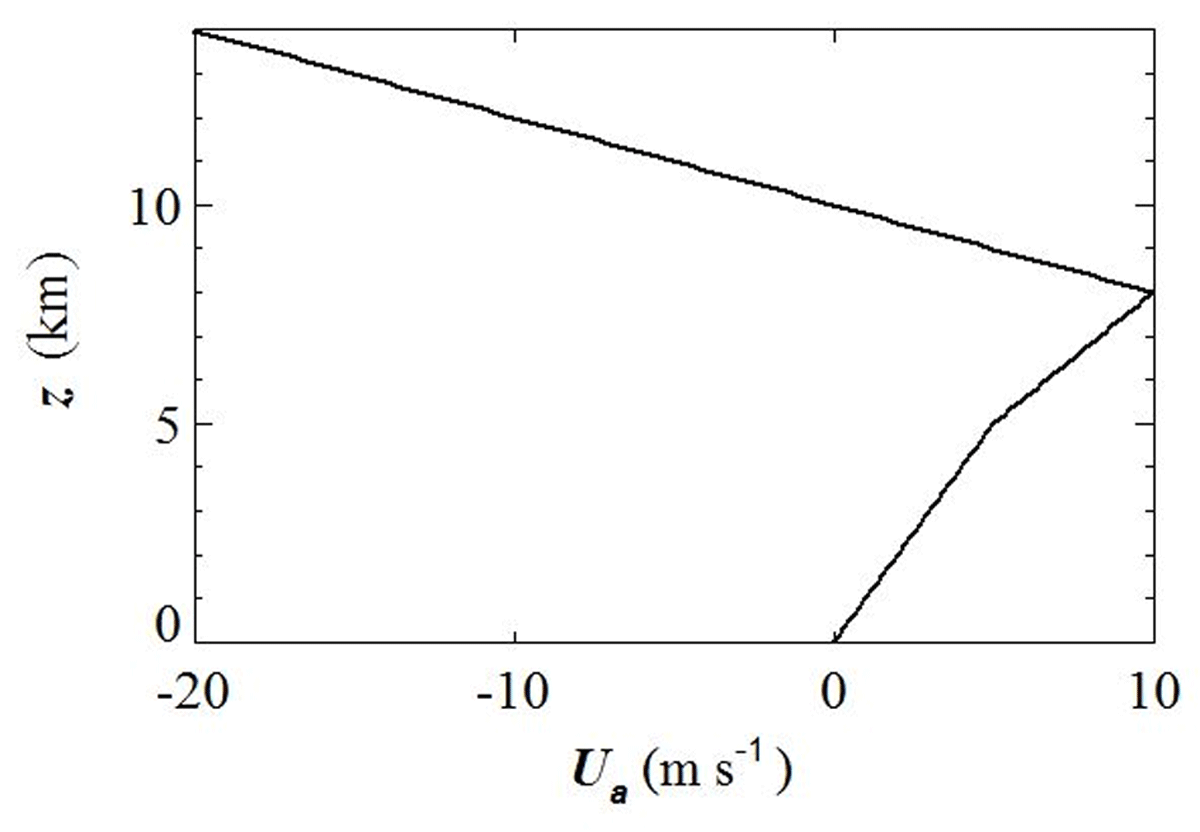
Figure 1
Atmospheric profile of horizontal wind.
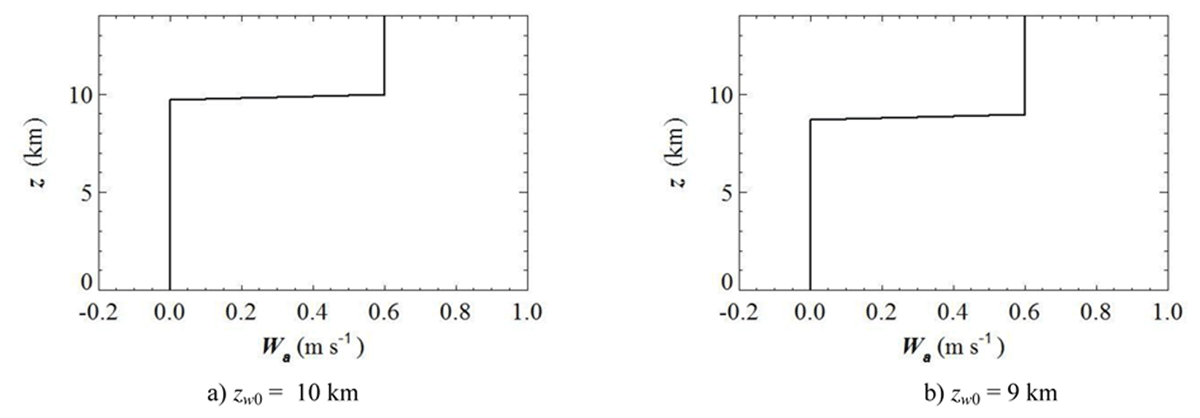
Figure 2
Atmospheric profiles of vertical wind.
The damping coefficient k is such that (Pruppacher & Klett 1978/1997):
Physically speaking, k is the reciprocal of a relaxation time τD for the drag force (Paoli & Shariff 2016). It involves the Reynolds number Re, defined from the velocity of the crystal relative to ambient air by:
with and .
Also needed are the drag coefficient CD, such that (Pruppacher & Klett 1978, 1997; Wang and Ji 1997):
the dynamic viscosity of air μa, such that, for –50 < T – Tr < 50 (Tr = 273.15 K) (Pruppacher & Klett 1978/1997):
and the mass density ρm of moist air (Picard et al. 2008; Nettesheim 2017):
When the crystal reaches its limit regime defined by vanishing vertical acceleration , we obtain, from Eq. (1b), the limit velocity:
defining the terminal fall velocity Wf ∞ by:
Thermodynamic data of atmospheric temperature and pressure are detailed analytically in App. A.2 and plotted in Figure 3. The trajectory is driven by the ambient motion and the variations of the crystal’s mass m, involved in the damping coefficient k, which evolves according to the process described in the following section.
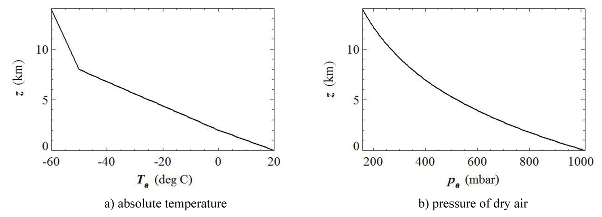
Figure 3
Atmospheric profiles of temperature and pressure of dry air.
2.2. Microphysics
2.2.1. Crystal mass
In this simplified approach, we consider an average ice crystal, once it has been generated by homogeneous nucleation in a highly ice-supersaturated environment (Si–1> 50%), and we follow its subsequent growth only by deposition of water vapour on its surface from an ambient medium slightly or moderately saturated with respect to ice (Köhler & Seifert 2015). Conversely, it loses matter by sublimation of ice into water vapour. In a model of cirrus including radiative transfer (Ramaswamy & Detwiler 1986), the growth of a crystal of 200 μm length is shown to reach an ambient ice supersaturation as small as 5% after 10 minutes. We shall show a posteriori that the oscillatory mode we put into evidence is likely to occur only if the ice supersaturation is of order of the radiative term (3 < R < 15%).
In the capacitance model, crystal’s mass growth is governed by the following equation with additional term R and factors fv and C accounting respectively for radiative transfer (R), ventilation (fv), and capacitance (C), namely (Houghton 1950; Mason 1953; Hall & Pruppacher 1976; Rogers 1979; Wu et al. 2000; Lebo et al. 2008):
subject to the initial condition:
where the initial volume V0 is estimated from Eq. (31a) below.
The saturation ratios Sl and Si of water vapour, over liquid water and ice respectively, are defined by (Pruppacher & Klett 1997; Bohren & Albrecht 1998):
The relative humidity Hl and Hi of water vapour, with respect to (wrt) liquid water and ice respectively, can be expressed, as recommended by the WMO (World Meteorological Organization), by the following expressions (Pruppacher & Klett 1978/1997; Bohren & Albrecht 1998):
The atmospheric moisture profiles are detailed in App. A.3, and plotted in Figure 4. All these altitude profiles of winds and humidity are consistent with radiosonde observations and input data used in realistic simulations with Eulerian numerical codes (Spichtinger 2014). The method of calculation of the partial pressure pv of water vapour from the given ambient moisture profile Hl is detailed in App. B, and the expressions of the saturation pressures pvsl and pvsi of water vapour over liquid water and ice are summarized in App. C.
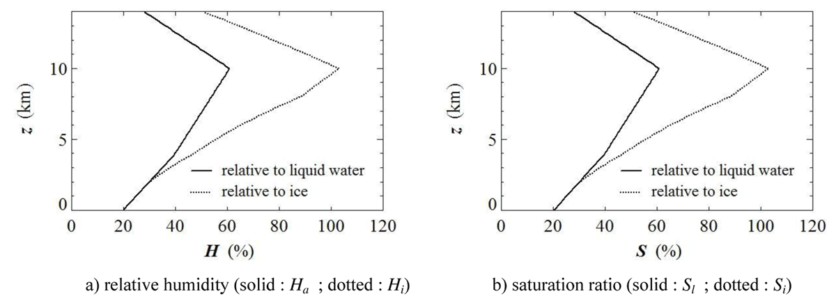
Figure 4
Atmospheric profiles of relative humidity and saturation ratios.
The saturation mixing ratio qs, necessary for the calculation of the Kelvin-Helmholtz criterion (Sect. 6.2), is such that:
The diffusivity of water vapour Dv in air and the heat conductivity of air Ka, involved in Eq. (10), are given by the following expressions (Rogers 1975)
Other parameterizations for Dv and Ka exist (see Zeng 2008), that are slightly different, in particular Dv being pressure-dependent, but they would give qualitatively the same results, though with different initial conditions. The ventilation coefficient fv is calculated using the following formulae, valid for column and plates in a laminar flow (Ji & Wang 1999; Liu et al. 2003a, b):
where the variable X, such that:
depends on Reynolds number Re defined by Eq. (4), and Schmidt number Sc defined by:
The factor Si–1–R playing a major role in Eq. (10) since it drives mass growth or decay according to its sign, we shall call it “driving factor” in the following.
2.2.2. Radiative transfer
The contribution of heat transfer in Eq. (10), appearing as a correction R to the ice supersaturation term Si–1, has been estimated using the formulation (Roach 1976; Wu et al. 2000; Lebo et al. 2008):
with the source term:
where Qabs denotes the absorption coefficient (Wu et al. 2000), Fu and Fd the upward and downward radiative flux densities respectively, A the crystal area, and Bi the black body radiative flux of crystal surface at temperature Ts:
Eq (19) has been used for fog and droplets (Roach 1976) and extensions to ice crystals in cirrus clouds (Stephens 1983; Wu et al. 2000; Gu & Liou 2000; Zeng 2008; Zeng et al. 2021) have been later widespread.
From the energy budget leading to Eq. (10), it is possible to calculate also the difference of temperature between the crystal’s surface (Ts), assumed homogeneous, and the ambient air (Ta):
We shall check a posteriori that this difference is small. Then Wien’s displacement law teaches us that the radiative transfer for a black body between – 20°C (253 K) and – 50°C (223 K) is in the range of wavelength 11–13 μm, i.e. infrared. Thus we shall consider infrared fluxes in Eqs. (20) and (23) (Stephens 1983). According to observational measurements (Inoue 1985) and theoretical background (Gierens 1994; Zeng 2008), we also assume that the emissivity ε of the crystal is equal to one.
Moreover we shall consider the transfer in the limit of short wavelength compared to the crystal dimensions, and therefore assume that Qabs ≈ 1 (Roach 1976; Liou 2002). It is convenient to express the radiative infrared ratio η as (Zeng 2008; Zeng et al. 2022):
and then recast Eq. (20) as:
Therefore, the crystal is subject to radiative cooling when η < 1, and to radiative warming when η > 1 (Zeng et al. 2021). If Fu and Fd are set to the following form at the top of the troposphere (Roach 1976):
then the ratio η becomes:
This is confirmed by the modelling of the parameter η we describe below.
Rather than modelling independently the radiative fluxes Fu and Fd, because that would involve too many additional degrees of freedom, it is usual to introduce an atmospheric ratio ηa as in Eq. (23), function of altitude. We shall derive an expression from models (Detwiler & Ramaswamy 1990; Zeng 2008) but consistent with observations (Paltridge and Platt 1981; Philipona et al. 2012), typical of a mid-latitude daytime atmosphere, that we detailed in App. A.4 and plotted in Figure 5.
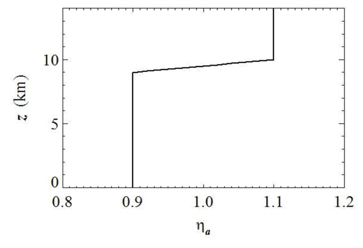
Figure 5
Atmospheric profile of atmospheric infrared ratio ηa.
The crystal-related η in Eq. (24) is related to the atmospheric ηa by a relationship of the form (Zeng 2018):
where the coefficient α depends on the shape of the crystal (Zeng 2018). We notice that when ηa = 1, then η = 1. and reciprocally, therefore radiative transfer cancels, whatever the shape could be. We estimated α from our various test cases in Sect. 5, and we found it to be in the range 0.1–0.4.
For the crystal to grow (), Eq. (10) shows that the following relation must be verified:
When η < 1, i.e. < 0, and therefore R < 0, we see from Eq.(28) that the saturation ratio Si need not be larger than one, and that an ice crystal can develop in a subsaturated environment (Hall and Pruppacher 1976). We shall experiment this situation with the oscillatory mode we found, in Case 3 relevant of uniform nighttime conditions (η = 0.9), which is detailed in Sect. 5.4.
Conversely, when η > 1, i.e. > 0, and therefore R > 0, we see likewise from Eq.(28) that the saturation ratio Si must be larger than one, and that an ice crystal will develop in a supersaturated environment. We shall experiment this situation for the oscillatory mode, in Case 2 relevant of uniform daytime conditions (η = 1.1), which is detailed in Sect. 5.3.
When η is altitude-dependent (Figure 5), we shall show that ice supersaturations as low as 3%, moreover consistent with observational statistics (Ovarlez et al. 2002; Spichtinger et al. 2004), can lead to ice crystal growth (Sect. 3.2.3).
In the present approach, the resulting variation of the ambient saturation ratio S due to crystal growth is not considered, since the crystal trajectory does not go twice through the same region of space, even in the oscillatory regime (Sect. 3.2.3). Moreover Kelvin’s effect due to surface tension has been neglected (Gu & Liou 2000). Of course, involving these effects would be a useful refinement in further developments.
2.2.3. Crystal shape
According to theoretical models (Kobayashi, 1961; St-Pierre and Thiérault, 2015) and observations (Heymsfield 1975a; Schmitt & Heymsfield 2007), hollow column and bullet-rosette are thought to be the crystal shapes most likely developing in cirrus clouds, most of them (50 to 80%) having hollow ends (Schmitt & Heymsfield 2007).
A first possible approach to connect crystal mass and dimensions consists in assuming a mass-length relationship, which is the way followed in the reference work (Heymsfield 1973; Heymsfield 1975c) and many others (Rogers 1979; Jensen et al. 2018; Mascio et al. 2017). Because of the crystal’s lacunarity, its mass density is then smaller than the actual density of solid ice (Cotton et al. 2013). A considerable amount of investigation has been devoted to the determination of the effective mass density of ice crystals encountered in cirrus clouds, both from in situ observational data (Heymsfield 1972; Heymsfield et al. 2002; Heymsfield et al. 2004; Schmitt & Heymsfield 2007; Cotton et al. 2013) and from laboratory experiments (Jensen & Harrington 2015). This is due to the fact that the cavities and hollow portions that are included in the effective volume make it larger than the actual volume.
An effective mass density ρie can be defined from the actual mass m and the maximum particle dimension Dm by the general expression (Cotton et al. 2013):
A more specific definition can be given on the basis of the volume of the solid hexagonal column (Fukuta & Takahashi 1999):
Dealing with hexagonal hollow columns, we shall use the latter definition.
An alternative approach consists in assuming a prevalent shape of the crystal, with a perfectly known geometry, so that its volume and surface area are easily calculated from its dimensions. Mass and volume are then connected to each other by means of Eq. (11) and (31) at each time, ρi being the actual mass density of ice (Fridlind et al. 2016). As far as ρi increases when temperature decreases (Pounder 1965), we shall adopt an average value: ρi = 920 kg m–3.
Leaving apart the bullet-rosette as too complex in a first step, we shall focus on the hexagonal hollow column. This kind of crystal has been thoroughly investigated (Chiruta & Wang 2005; Fridlind et al. 2016; Zeng 2018), and it has been shown that the crystal’s volume and area can be simply expressed as (Chiruta & Wang 2005; Chen & Wang 2009):
The shape of a hollow column with hexagonal cross section, drawn after Chen and Wang (2009), is shown in Figure 6. The core bulk of half-length cB, is limited by two pyramidal hollow ends of depth c–cB.
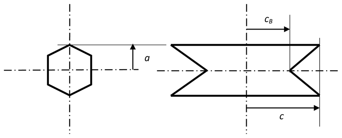
Figure 6
The shape of the mean crystal (meridian and axial cross sections) (after Chen and Wang, 2009).
In their analytical model of crystal growth (Chen & Wang 2009), these authors assume that, during the growth, the parameter cB is subject to one the conditions:
We shall here extend this assumption and quantify the hollow portion of the crystal by a hollowness factor (Schmitt & Heymsfield 2007) denoted here ψ:
We shall keep cB constant, equal to its initial value: cB0 = (1–ψ0) c0. For crystals longer than 100 μm, we shall set: ψ = 0.8 (Schmitt & Heymsfield 2007).
A further simplification consists in assuming that either the radius a is constant (Harimaya 1968, Chen & Wang 2009) or a and c are connected by some width-length relationship (Chen & Wang 2009; Pruppacher & Klett 1978). Adopting the first assumption, we found that the aspect ratio ϕ:
reaches large values (ϕ > 30) as soon as the saturation exceeds 130%, relevant of thin needles, inconsistent with observations. Therefore, we adopted the second assumption, and assume thereby that, for hollow columns, the aspect ratio ϕ is constant during the motion. The value ϕ = 2 was found for columns with c < 150 μm from in situ measurements (Heymsfield 1972; Um et al. 2015). Therefore, using Eq. (31a,b) and the definition of ϕ we are led to a third-degree equation for a:
As the crystal evolves, its mass m changes, and its volume V is calculated by the relation:
The crystal’s shape being significantly different from a sphere, it is useful and usual to define the mass equivalent diameter Di and radius ri = Di/2 of the crystal as those of the sphere with the same volume V as the crystal, namely:
or, using Eq. (36):
Alternately, by setting a maximum particle size Dm = max(2a,2c), as the larger of the two dimensions 2a and 2c (that is 2c if ϕ > 1 or 2a if ϕ < 1) following the general definition (29) and using Eq. (36), we could also define an effective mass density ρie such that:
Following the more specific definition (30), we obtain the expression (Fukuta & Takahashi 1999):
which will yield values smaller than the actual density ρi. The first definition (Eq. (39)) overestimates the actual volume, and therefore, it underestimates ρie, yielding values as low as 200 kg m–3 found in observations of complex particles or aggregates (Heymsfield et al. 2004). The second definition (Eq. (40)) yields values in better agreement with observations of simple shapes (Miller & Young 1979; Schmitt & Heymsfield 2007), and we shall follow its variation during the motion of the crystal.
For a hollow column, the capacitance C appearing in Eq. (10) can be written (Chiruta & Wang 2005):
using the aspect ratio ϕ defined above (Eq. (34)). Moreover, we shall assume that the ventilation coefficient defined by (16) accounts for the different orientations of the crystal during its motion. A detailed account of the flow characteristics around columns and plates with estimation of torques based on Navier-Stokes equations teaches us that the Reynolds number ranges from 2 to 70 (Hashino et al. 2014). Lidar observations show that plane crystals have mainly horizontal orientation during free fall, with a maximum tilt angle of 0.3 degrees (Thomas et al. 1990). The particle radius ri is set equal to Di/2 in Eqs (3) and (19), and to Di in Eq. (4) as a possible alternative definition of Reynolds number (Pruppacher and Klett 1997). While it is easy to define an equivalent diameter for liquid spherical particles, this is quite difficult for ice crystals (McFarquhar & Heymsfield 1998). Thus, large discrepancies occur for radii larger than 50 μm, so that we shall keep the above convention. Nevertheless, we shall also display the half-length c in the result of calculations.
3. Solutions
3.1. Numerical method
The differential system composed of Eqs. (1a, b) and (10) is a Liénard system (Perko 1990), that we discretized with finite differences, and using an explicit Euler scheme such that, at any time tn = n ∆t, we write the velocity components of the average crystal’s center of mass as:
its rectangular coordinates as:
and its mass as:
where Tn = Ta(zn) and Sn = Si(zn) are calculated from the data detailed in App. A. Eqs. (42), (43), and (44) constitute a set of strongly coupled nonlinear equations.
Because the radiative correction R and the capacitance C (Eqs. (19) and (41) respectively) are dependent of the axial size c, we also need to recalculate Vn+1 from mn+1 using Eq. (36):
and then cn+1 from Eq. (31a,b) if a is constant (a = a0):
or solving Eq. (35) for an+1 if ϕ is constant (ϕ = ϕ0):
We neglect the variation of the gravity field g with altitude, between approximately 7 and 10 km height, the Coriolis force, and the influence of the column orientation on the ventilation coefficient fv.
Below is given a detailed account of the two regimes or modes we found with standard initial conditions. Two special sections will be devoted respectively to the sensitivity of various parameters (lifetime, period, amplitude…) to the crystal’s initial size a0 (Sec. 4) and to the impact of radiative transfer (Sect. 5).
3.2. Results
3.2.1. Data and displays
In this section the simultaneous integration of the discretized differential system composed of Eqs. (42) to (45) and (47) subject to the initial conditions of Table 2 (Case 0) is carried on with the aspect ratio ϕ and the core half-length cB kept constant at each time step: ϕ = ϕ0 and cB = cB0. We obtain a dual mode composed of a steady well-developed, non-oscillatory, cirrus uncinus (hooked cap + trail) with a high-base updraft, and an oscillatory counterpart associated with a low-base updraft.
Table 2
Parameters of test-cases/numerical experiments.
| CASE NB | 0 | 1 | 2 | 3 |
|---|---|---|---|---|
| NET RAD. TRANSF. | R ≠ 0 | R = 0 | R ≠ 0 | R ≠ 0 |
| Parameter | η(z) ϕ = ϕ0 cB = cB0 | η = η0 = 1 ϕ = ϕ0 cB = cB0 | η = η0 ≠ 1 ϕ = ϕ0 cB = cB0 | η = η0 ≠ 1 ϕ = ϕ0 cB = cB0 |
| Modes | Steady – Osc | Steady – Osc | (Steady) – Osc | (Steady) – Osc |
| Life time | 5 h/40 h | 5 h/40 h | 4 h/40 h | 4 h/40 h |
| ∆t (s) | 0.02/0.04 | 0.02/0.04 | 0.02/0.04 | 0.02/0.04 |
| x0 (km) | 2 | 2 | 2 | 2 |
| z0 (km) | 10 | 10 | 10 | 10 |
| u0 (m s–1) | 0 | 0 | 0 | 0 |
| w0 (m s–1) | 0.6 | 0.6 | 0.8 | 0.8 |
| a0 (μm) | 51.1 | 50.17 | 52.0 | 50.2 |
| c0 (μm) | 102.2 | 100.34 | 104.0 | 100.4 |
| ϕ0 | 2.0 | 2.0 | 2.0 | 2.0 |
| ψ0 | 0.80 | 0.80 | 0.80 | 0.80 |
| cB0 (μm) | 20.44 | 20.068 | 20.80 | 20.08 |
| m0 (μg) | 0.935 | 0.885 | 0.986 | 0.887 |
| C0 (μm) | 88.6 | 86.9 | 90.1 | 87.0 |
| D0 (μm) | 125 | 122 | 127 | 123 |
| ρie0 (kg m–3) | 675 | 675 | 675 | |
| η | 0.9 ≤ η ≤ 1.1 | 1 | 1.1 | 0.9 |
| zη0 (km) | 9 ≤ z ≤ 10 | 0 – 11 | 0 – 11 | 0 – 11 |
| Wa0 (m/s) | 0.6 | 0.6 | 0.8 | 0.8 |
| zW0 (km) | 10/9 | 10/9 | 10/7 | 10/7 |
| Ha3 | 0.61 | 0.61 | 0.68 | 0.68 |
| zH3 (km) | 10 | 10 | 10 | 10 |
| zmax0–z0 (m) | 102 | 144 | 468 | 542 |
| z∞(km) | 9.63 | 9.58 | 8.58 | 8.3 |
| P (hour) | 10.2 | 8.87 | 7.8 | 6.8 |
| Λ (km) | 69.8 | 64.8 | 200 | 200 |
| Cp (m s–1) | 1.85 | 2.03 | 7.1 | 8.2 |
| ζ | 0.019 | 0.015 | 0.021 | 0.011 |
For each of the two selected modes are displayed crystal trajectory z(x), hodograph or phase portrait w(u), abscissa and altitude, free fall speed Wf, dimensions (a, c, cB), mass equivalent diameter Di, dynamic viscosity of air μa, hollowness factor ψ, effective mass density of crystal ρie, drag coefficient cD, Reynolds number Re, damping coefficient k, temperature difference Ts–Ta between ambient air and crystal surface.
Two kinds of dual solutions are obtained, depending on the altitude zw0 of the updraft base, other things being unchanged. Nevertheless, these two solutions are obtained after a minute fitting of the crystal initial half-width a0, the wind velocity amplitude and the updraft intensity, altitude and thickness, in narrow ranges. This behaviour is mostly conditioned by the temperature and humidity profiles we chose (App. A), which are characteristic of a mid-latitude cirrus background. We also show phase relationships in the various time profiles of the damped oscillator solution.
3.2.2. Non-oscillatory mode
When the base of the updraft lies at an altitude of 10 km (Figure 2a), the trajectory looks like that obtained from the shape of an average cirrus uncinus, with a hooked head and a trail or virga (Figure 7a), consistently with a conceptual view (Heymsfield 1975b) and the description given by the International Cloud Atlas (WMO 1975). The head is similar to the upper part of a cirrus uncinus as observed during the FIRE IFO II experiment, and reported later (Sassen & Krueger 1993).
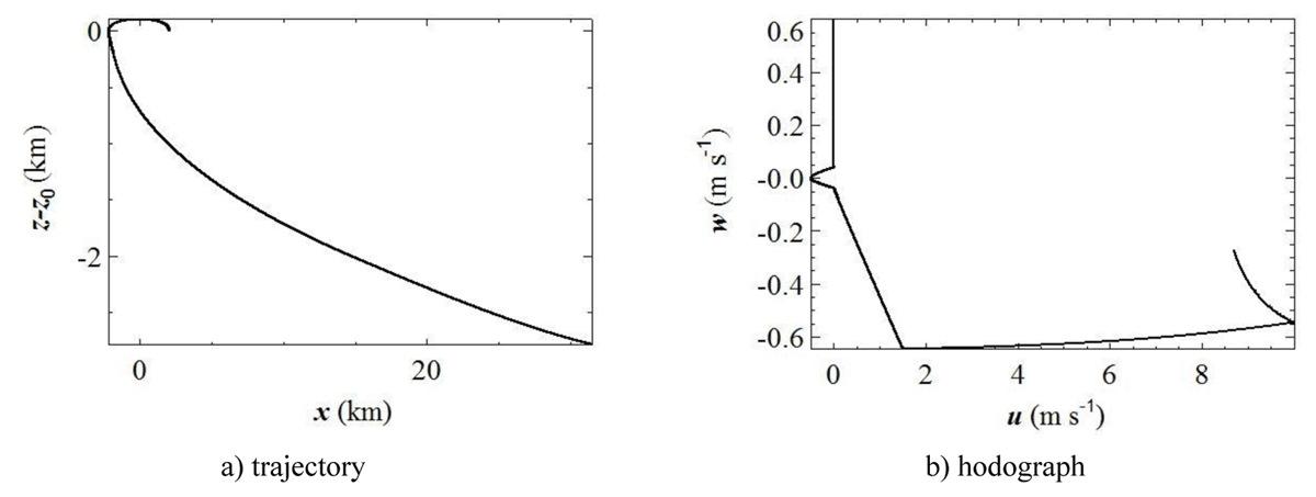
Figure 7
Profiles of the parcel trajectory and hodograph (z0 = 10 km; zw0 = 10 km).
The trail or virga, referring to the curved shape with a dot at the origin (similar to the French word “virgule” meaning comma), is seen in the lower part. Its physical nature has been subject to a controversy (Fraser & Bohren 1992; Sassen & Krueger 1993). Actually, in our simplified approach, the crystal sublimation takes place in the virga. Along the trajectory, the maximum height (where dz/dt = 0) is reached after approximately 1.5 hours (Figure 8b), and the extremum (where dx/dt = 0) after 3.3 hours (Figure 8a).
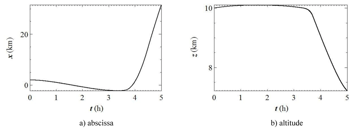
Figure 8
Time profiles of abscissa and altitude (zw0 = 10 km).
The hodograph (Figure 7b) has no periodic branch and tends toward free fall with entrainment by horizontal wind. Our vertical velocities are smaller than reported values (Heymsfield 1975a), consistently with the fact that we assume a weaker updraft (0.6 m s–1 instead of 1 m s–1), but they are in good agreement with FIRE observations (Gultepe et al. 1990).
The scale lengths are compatible with our calculated shape and the integration runs over 5 hours, a duration that represents about 1/6 of a typical cirrus uncinus lifetime (Luo & Rossow 2004). With a constant time step ∆t = 0.02 s, 900000 time steps are necessary.
The time profiles of abscissa and altitude (Figure 8) shows that the crystal spends much time in the head where it grows for about three hours, and then decays rapidly, consistently with its mass (Figure 11a). The profile of abscissa (Figure 8a) shows a minimum at 3.3 hours, reached at the left-most point of the trajectory (Figure 7a), where the crystal is pushed by the horizontal wind (Figure 1) directed to the left (Ua < 0). Afterwards, the crystal falls down in the decay phase following the trail.
The profile of free fall speed Wf (Figure 9a) is a good test because it is similar to that obtained with the analytic model developed in App. D.1. The estimate of the theoretical time duration obtained there is consistent with the 5 hours reached here. We find typical values of Wf in the range 25–65 cm s–1 that are in good agreement with observations of downdrafts in cirrus clouds (Heymsfield 1975b), as well as laboratory and field measurements (Heymsfield & Westbrook 2010) and measurements in synoptic cirrus (Mishra et al. 2014).
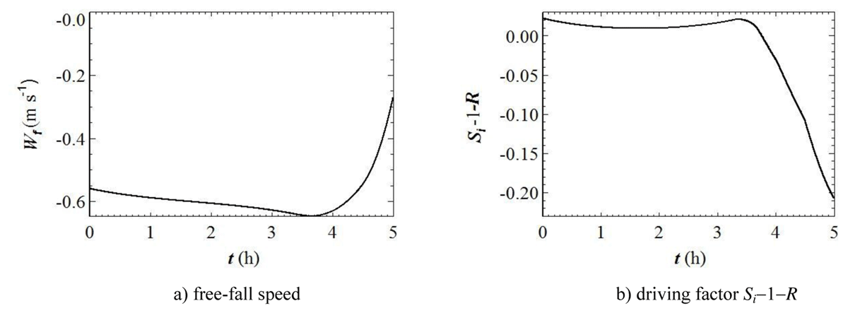
Figure 9
Time profiles of free-fall speed Wf and driving factor Si–1–R (zw0 = 10 km).
The variation of ice supersaturation Si –1 (Figure 10a) is roughly stationary, with a local minimum coincident with the height maximum (t ≈ 1.5 h) and positive between 2 and 3% during the growth phase until 3.4 hours. Then it decreases, becomes negative (t ≈ 3.75 h) in the decay phase, goes down to –20%, consistent with observational data fitted with a microphysics model (Khvorostyanov & Curry 2008).
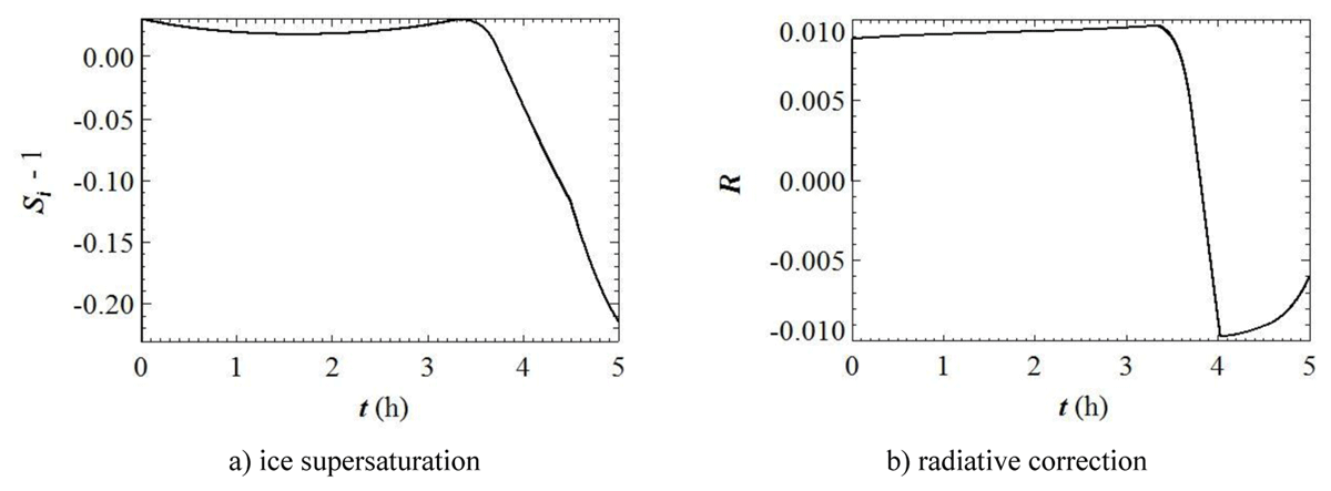
Figure 10
Profiles of ice supersaturation Si–1 and radiative correction R (zw0 = 10 km).
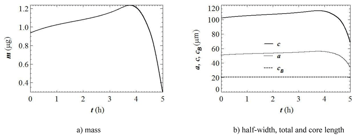
Figure 11
Profiles of crystal’s mass and dimensions (zw0 = 10 km).
The radiative correction term R (Figure 10b) is positive and slightly increasing, amounting to 1%, in the growth phase and becomes negative (t ≈ 3.75 h), synchronously with Si–1, then decreases to nearly –1% in the decay phase. Therefore this contribution is smaller than the supersaturation (Si –1 ≈ 3%), and as shown by Eq. (10), its effect counterbalances supersaturation in the heated growth phase (R > 0) and contributes in the cooled decay phase (R < 0) to lengthen the crystal’s life time. Consequently, the driving factor Si–1–R (Figure 9b) is slightly smaller than the supersaturation Si–1.
The crystal mass m (Figure 11a) is the variable coupled with position (x, z) and its profile shows an inflexion point at the altitude maximum (t ≈ 1.5 h), then reaches a maximum (m ≈ 1.2 μg) at t ≈ 3.75 hours and decays afterwards down to approximately 0.3 μg. The dimensions a and c (Figure 11b) reach maxima at the same time (t ≈ 3.75 h), and then decrease to 35 μm and 70 μm respectively, satisfying the initial aspect ratio (ϕ = 2). According to our assumption, the core half-length cB remains constant during the motion. The total length 2c is of same order as modelled by other researchers (Jensen et al. 2018).
The mass equivalent diameter Di (Figure 12a) has a maximum (Di ≈ 137 μm) at the same time (t ≈ 3.75 hours), corresponding to a distance of 400 m (Figure 8a), quite consistently with a simple former model (Harimaya 1968). The value Di ≈ 85 μm is reached in the virga after 5 hours, in good agreement with observations at similar temperatures (Baum et al. 2000; Kuhn & Heymsfield 2016). Dynamic viscosity (Figure 12b) is, together with the diameter Di (or radius ri = Di/2), a key parameter that scales the drag force (Eq. (3)) and Reynolds number (Eq. (4)). It is nearly constant in the head during 3.6 hours, and then it increases in the trail.
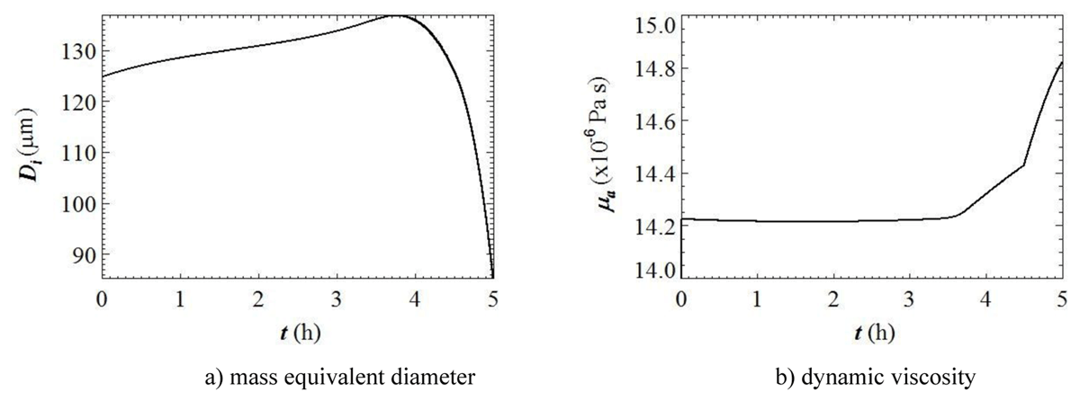
Figure 12
Profiles of mass equivalent diameter and dynamic viscosity (zw0 = 10 km).
The hollowness factor ψ (Figure 13a) increases during the growth phase, reaching a maximum close to 0.82 at 3.75 h, approximately like mass, and then decreases down to nearly 0.70. This is consistent with the opposite variation of effective mass density (Figure 13b). Actually, ρie, as calculated from Eq. (40), reaches a minimum when Di is maximum (t ≈ 3.75 h) and afterwards increases to large values. The range 670–705 kg m–3 covered during crystal motion is slightly smaller than values amounting to 800 kg m–3 published for bullet shapes (Schmitt and Heymsfield 2007).
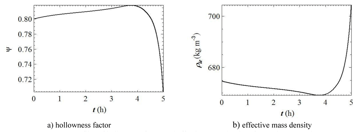
Figure 13
Profiles of hollowness factor and effective mass density of crystal (zw0 = 10 km).
The drag coefficient CD (Figure 14a) reaches a minimum at 4.2 h, later than the mass maximum (Figure 11a), but expectingly in phase with the maximum of Reynolds number Re at the same time (Figure 14b). The ranges covered by CD (9–25) and Re (1–3) are perfectly confirmed by numerical and laboratory experiments (Wang & Ji 1997).
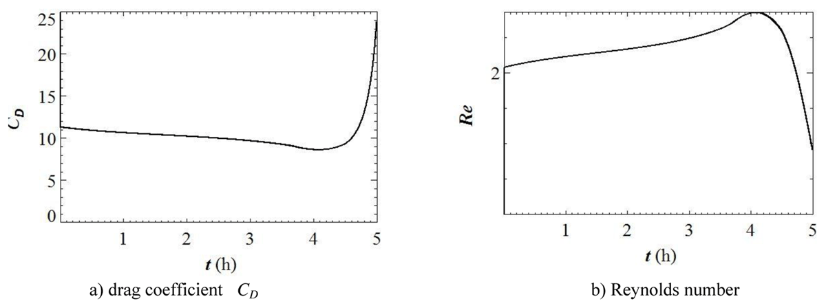
Figure 14
Profiles of drag coefficient and Reynolds number (zw0 = 10 km).
The damping coefficient k (Figure 15a) is minimum at 3.75 hours and it increases by 50% in the final phase. It amounts to 15–20 s–1 and therefore the quantity k ∆t is maintained in the range 0.3–0.6 thus ensuring stability of the algorithm (Eqs. (42)). The temperature difference Ts–Ta (Figure 15b) is very small and positive in the heated growth phase (Ts–Ta < 0.01 K), then it becomes negative and increases in magnitude (Ts–Ta < 0) in the cooled decay phase, though remaining smaller than 0.1 K, consistently with published results (St-Pierre & Thiérault 2015).
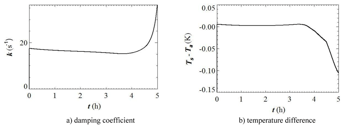
Figure 15
Time profiles of damping coefficient and temperature difference ice-air (zw0 = 10 km).
We can notice that the angular point appearing on certain profiles is due to the angular point present on the theoretical piecewise temperature profile (Figure 3a) with coordinates: z = 8 km, Ta = –50°C. It affects quantities depending directly of the temperature (dynamic viscosity, temperature difference…), and consequently the velocity components (hodograph). In contrast, the trajectory is everywhere differentiable because of the smoothing of coordinates (x,z) due to the time integration of velocity components (u,w).
3.2.3. Oscillatory mode
When the base of the updraft is lowered down to an altitude of 9 km (Figure 2b), other parameters being unchanged, the trajectory is subject to a damped oscillation (Figure 16a). After the hooked head is formed with approximately a hundred meter vertical extension, like in the previous steady, non-oscillatory mode (Sect. 3.3.2), the crystal parcel follows a periodic motion, whose wavelength Λ and period P are approximately 70 km and 10.5 hours respectively. The amplitude of height oscillations is about 400 m at the beginning, and it decreases afterwards (Figure 17b).
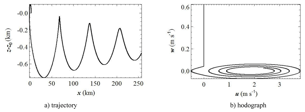
Figure 16
Profiles of the parcel trajectory and hodograph (z0 = 10 km; zw0 = 9 km).
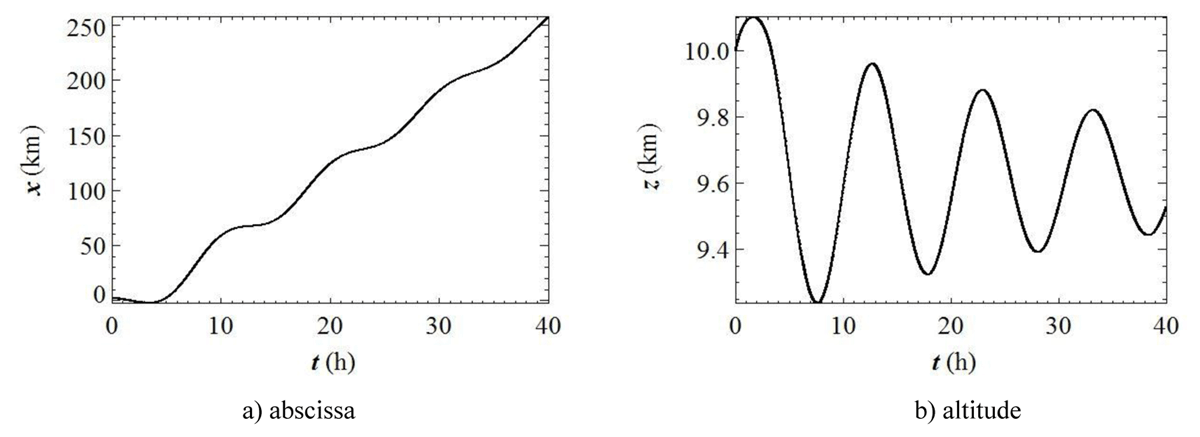
Figure 17
Time profiles of abscissa and altitude (zw0 = 9 km).
Owing to the mass loss of the crystal, which induces variations of the damping coefficient k (Figure 24a) or equivalently of the viscous drag (Figure 23a), the updraft acts in the bottom part of the trajectory at an altitude of 9.2 km, that is 200 m above the base (zw0 = 9 km), causing the parcel to lift again, like in cumulus models (Grabowski 1993). The crystal bounces on the updraft base like a ball on a rigid floor, except that the crystal equilibrium altitude is not the lower attained level (z–z0 ≈ –0.75 km in Figure 16a), but an intermediate height, unlike the ball that stabilizes at the floor level.
Let us examine the limit focus of the hodograph (Figure 16b) which is composed of a straight line followed by a hook corresponding to the head, and afterwards of a spiral trajectory winding one turn more at each period. The phase velocity Cp corresponding to the period P and wavelength Λ is defined by:
that is, numerically: Cp = 70 × 103/(10.5 × 3600) ≈ 1.85 m s–1. Now, let us write the condition for the fixed point:
and using Eqs. (1a, b) and neglecting the buoyancy force, we obtain:
The fixed point satisfies the additional condition:
and this finally leads to:
Extrapolating the hodograph spiral (Figure 16b) shows that the horizontal velocity tends towards u∞ = 1.85 m s–1 approximately. We can then estimate the wind speed at the limit height z∞ ≈ 9.63 km (Figure 18a) using Eqs. (68) in layer III: Ua(z∞) = –30 –5(9.63–16) = 1.85 m s–1. This confirms the value given by the cycle focus (Ua(z∞) = u∞). Moreover, this limit velocity is very close to the phase speed of oscillations Eq. (48), which is approximately 1/10 that of gravity waves.
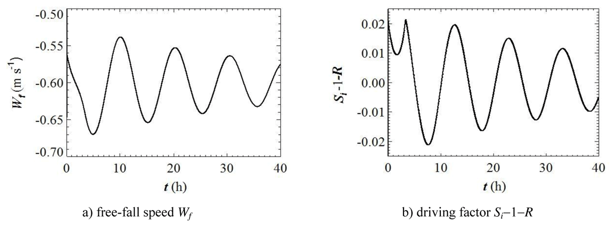
Figure 18
Time profiles of free-fall speed Wf and driving factor Si–1–R (zw0 = 9 km).
It is noteworthy that the maxima along the trajectory (Figure 16a) are sharp at the beginning and tend to become blunter and blunter, while the minima have nice round shapes all along the motion, like the extrema of other parameters displayed in the following. This is due to the fact that the abscissa (Figure 17a) is not a linear function of time, but has a periodic component of decreasing amplitude superimposed on a secular variation (of order Cp t; see below).
As can be clearly seen on the time profile of altitude (Figure 17b), the limit height (z∞ ≈ 9.63 km) is slightly larger than the updraft base (9 km). It is in good agreement with the theoretical model of damped harmonic oscillator built in App. D.2 on the same period and a matched damping ratio (Figure 41a). As it was noticed, the abscissa x has a wavy profile (Figure 17a), and being coupled to altitude z through Eq. (1), it is in quadrature with z, since its quasi-horizontal inflexion points are coincident with maxima of z, and its oblique inflexions are in phase with minima of z. The slope of the straight line passing through these inflexion points is approximately equal to the phase speed Cp and the limit velocity u∞.
The time profile of fall speed Wf (Figure 18a) oscillates with the same characteristics as the trajectory, and it tends towards the terminal value Wf ∞ ≈ – 0.6 m s–1, which compensates the updraft (Wa = 0.6 m s–1), and thus sustains the parcel oscillation. We can notice that, up to 10 hours, its beginning portion quite consistently looks like the theoretical profile relative to the steady mode shown in App. D.1 (Figure 38).
The ice supersaturation Si –1 (Figure 19a) shows damped oscillations with the same period and it does not tend towards zero, but towards 0.25% with increasing time. Its amplitude is initially small (3%) but larger than the radiative correction (0.75%). Moreover, Si –1 and R are in phase with altitude (Figure 17b) and in quadrature with mass (Figure 20a). At infinity they both tend towards 0.25%, and consistently the driving factor Si–1–R (Figure 18b) tends towards zero. We shall examine further below (Sect. 5) the relation between Si–1 and R for the oscillation to develop.
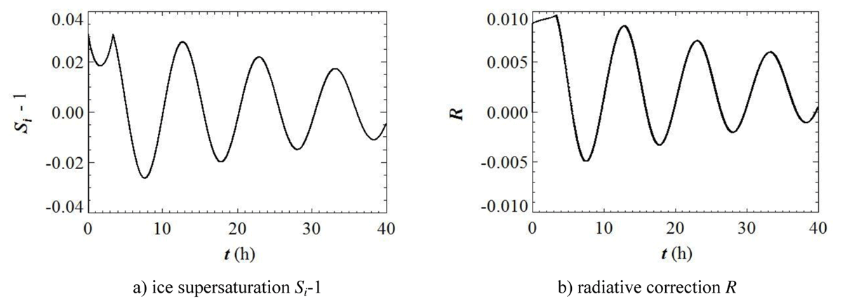
Figure 19
Time profiles of ice supersaturation Si-1 and radiative correction R (zw0 = 9 km).
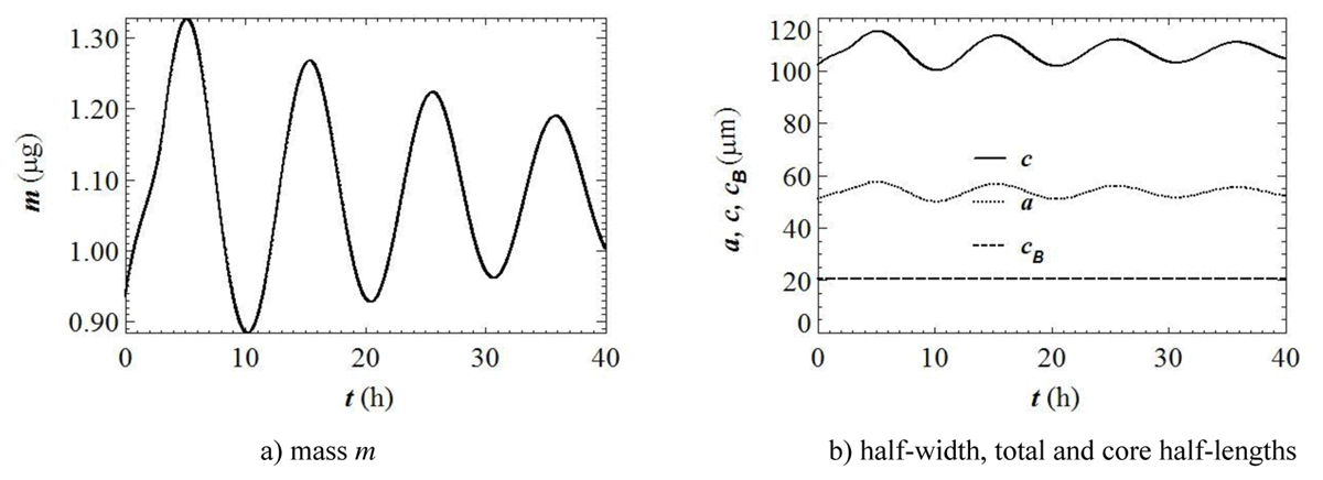
Figure 20
Time profiles of mass m and dimensions a, c, cB (zw0 = 9 km).
Crystal mass (Figure 20a) is the variable coupled with position (x, z), and careful examination of its profile compared to that of attitude z (Figure 17b) and supersaturation (Figure 19a) shows that they are in phase quadrature. The dimensions a and c (Figure 20b) naturally show damped oscillations, in phase with mass. The half-length c tends towards a limit c∞ ≈ 108 μm at infinity, which is larger than the initial one (c0 = 82.95 μm).
The mass equivalent diameter (Figure 21a) oscillates in phase with the fall speed and half-length c, and it tends towards a limit value, approximately 131 μm. Because of its definition, Eq. (38), it is naturally in phase with mass (Figure 20a). Dynamic viscosity (Figure 21b) is an important parameter that scales the viscous drag. We understand from its being in phase opposition with altitude (Figure 17b), that when the crystal reaches the top of a spatial period, gravity predominates over viscous drag, and the crystal falls down. When it reaches the bottom of a period, the situation is reversed: viscous drag predominates and the crystal is pushed up.
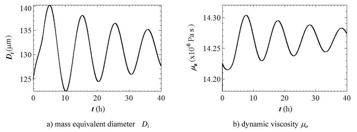
Figure 21
Time profiles of mass equivalent diameter and dynamic viscosity (zw0 = 9 km).
The core half-size cB being kept constant during the motion (Figure 20b), the hollowness factor ψ (Figure 22a) oscillates with a small amplitude (≈2%) in phase with c, and it tends towards a limit value (ψ∞ ≈ 0.81) slightly larger than its initial value (ψ0 = 0.80). The crystal’s effective mass density as calculated from Eq. (40), shows oscillations (Figure 22b) in phase with Wf, and phase opposition with ψ and Di. It tends towards the asymptotic approximate value 671.5 kg m–3 approximately.
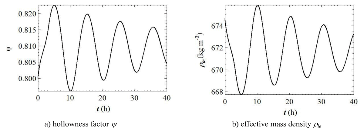
Figure 22
Time profiles of hollowness factor and effective mass density of crystal (zw0 = 9 km).
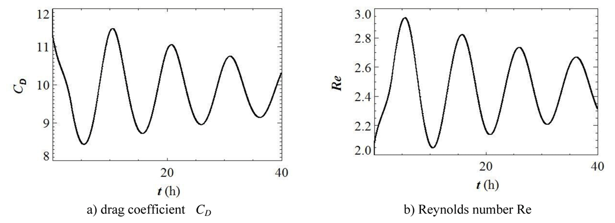
Figure 23
Time profiles of drag coefficient CD and Reynolds number Re (zw0 = 9 km).
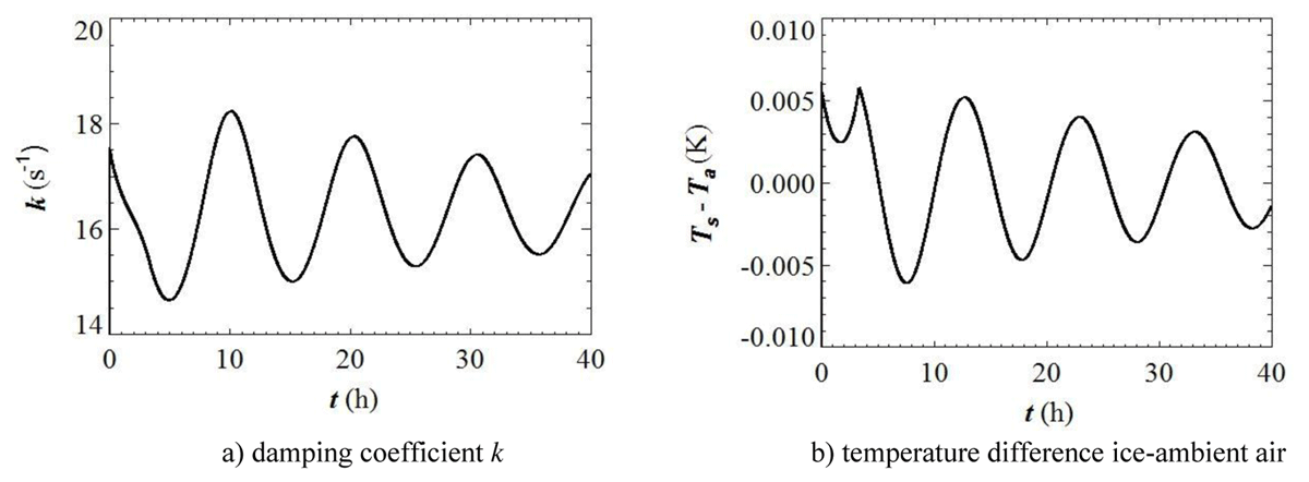
Figure 24
Time profiles of damping coefficient k and temperature difference ice-ambient air (zw0 = 9 km).
The drag coefficient CD (Figure 23a) oscillates also at the same frequency and wavelength, in phase opposition with Reynolds number Re (Figure 23b). These two parameters are respectively comprised in the ranges 8.5–11.5 and 2–3 and tend towards 10 and 2.45 at infinity. Like in the non-oscillatory mode (Sect. 3.2.2), the ranges covered by CD and Re are in good agreement with numerical and laboratory experiments (Wang & Ji 1997). Nevertheless, probably because CD and Re involve the mass variation through the mass equivalent radius (Eq. (4)), they are phase quadrature with altitude.
The damping coefficient k (Figure 24a) oscillates roughly between 15 and 18, and tends towards the value k∞ ≈ 16.5 s–1, which is connected to Wf ∞ (≈ 0.6 m s–1) through Eq. (9). The oscillation of the temperature difference between the crystal’s surface and the ambient air (Figure 24b) tends towards zero as time tends to infinity, i.e. the surface temperature tends towards the ambient temperature Ta corresponding to the limit height z∞ ≈ 9.63 km.
In the next sections we shall focus on the impact of crystal’s initial mass or size (Sect. 4) and radiative transfer (Sect. 5) on the trajectory, as primary causes of spreading of the cirrus structure.
4. Sensitivity to crystal size
4.1. Non-oscillatory mode
Below a critical size (a0 < 53.4 μm), the crystal parcel is lifted, brought along towards negative x, and does not fall down below its generating level. On the opposite, above a size threshold (a0 > 53.4 μm), the parcel is not lifted and directly falls down below its generating level, yielding only the virga without hooked head.
Looking in detail the situation of the parcel at horizontal distances of 10 and 20 km gives some insight into the crystal’s history. The falling heights z10 – z0 and z20 – z0 (Figure 25a) are maximum when a0 ≈ 53.4 μm and then decrease quite linearly as function of a0. The spans of z10 – z0 and z20 – z0 in the range 55–100 μm reach 600 m and 2 km respectively, and they give an idea of the trail thickness that is consistent with published results (Sunilkumar & Parameswaran 2005) for moderately cold cirrus (–75°C < T–Tr < –50°C). Colder cirrus (–85°C < T–Tr < –75°C) at higher altitudes are thinner.
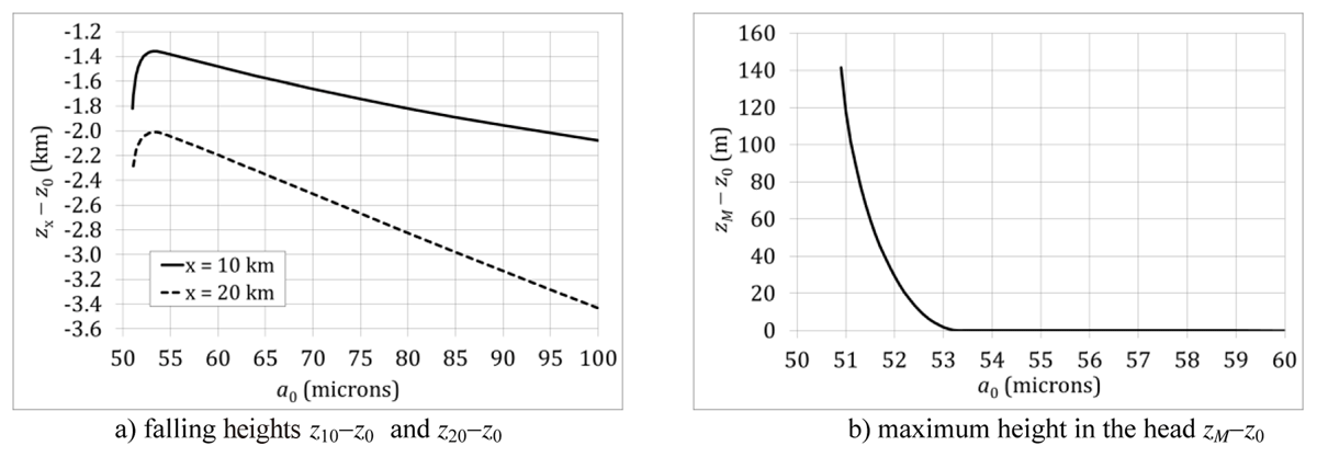
Figure 25
Profiles of falling height z20–z0 and maximum height in the head zM–z0 as functions of crystal half-width a0 (zw0 = 10 km).
Interestingly it appears that the relative maximum height zM – z0 reached at the top of the hook (Figure 25b) plotted as a function of a0 comes to zero at a0 ≈ 53.3 μm, indicating that a hook does not form for larger sizes. In the opposite, when the crystal is smaller, a head develops up to more than 100 m above the initial position, and as expected, the lighter it is, the higher it is lifted.
Simulations of cirrus clouds (Dobbie & Jonas 2001) in presence of radiative cooling (RC) show that IWP decay is achieved in approximately 5 hours without RC whatever the cloud thickness, and this lifetime is increased for thin clouds up to more 7 hours with RC.
The transit times t10, t20 at the abscissae x = 10 and 20 km plotted as a function of a0 (Figure 26a) reach several hours for small crystals (a0 < 52 μm) and shorten to less than one hour for large crystals (a0 > 55–65 μm).
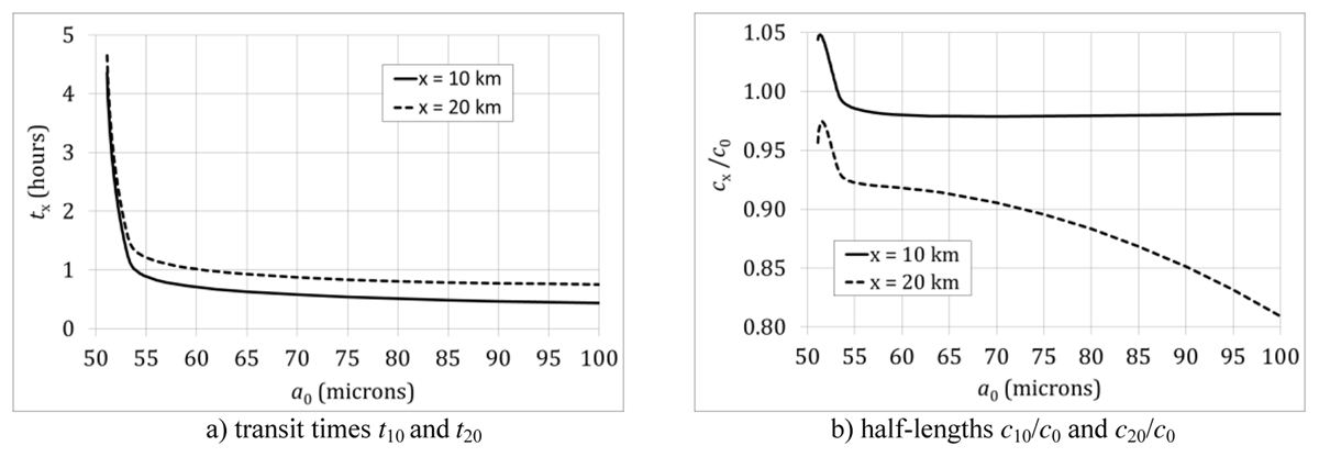
Figure 26
Profiles of transit times t10, t20 and half-lengths c10/c0 and c20/c0 as functions of crystal half-width a0 (zw0 = 10 km).
The half-lengths c10 and c20 at the same times, normalized to the initial value c0 and plotted as functions of a0 (Figure 26b) show an interesting behaviour. The profiles have a sharp peak at approximately a0 ≈ 51.5 μm, and then decrease with inflexion points corresponding roughly to the maxima of the falling height profiles (Figure 25a). Then, c10/c0 is nearly constant, while c20/c0 decreases nonlinearly down to 80%. Thus, the crystal size changes little up to 10 km and undergoes its major decay at 20 km by more than 10% according to its initial size in the range 55–100 μm. Unlike the falling height, the crystal decay is a strongly nonlinear function of size, reflecting the complexity of the microphysical processes involved in the model despite its many simpliflying assumptions.
4.2. Oscillatory mode
We shall examine the first three (exceptionally four) extrema in the trail. Like in Sect. 4.1, below a critical size (a0 < 50.9 μm), the crystal is lifted, brought along towards negative x, and does not fall down below its generating level. On the opposite, above a threshold (a0 ≈ 56 μm), a transition occurs at the first maximum (in the x-range 25–40 km) where the horizontal velocity u vanishes because of the crystal becoming too heavy and the damping passing through an inflection point. Then horizontal velocity u changes sign and a loop forms, grows until the crystal is trapped in the first period, and the motion loses its spatial periodicity.
From the transit times at the first three minima (tmin1, tmin2, tmin3) and maxima (tmax1, tmax2, tmax3) we can calculate two estimates Pmin and Pmax of period by the formulae:
and plot the results as functions of a0 (Figure 27). Ne notice that the average involving the middle minimum or maximum would yield the same result, since: (tmin3–tmin2)+(tmin2–tmin1) = tmin3–tmin1, and: (tmax3–tmax2)+(tmax2–tmax1) = tmax3–tmax1. It is noteworthy that the period is nearly independent of crystal size a0 in the range 51–56 μm and the two curves for Pmin and Pmax are nearly coincident within 10–3. Estimates from these two plots are consistent with the value found in Sect. 3.2.3. The steepening at a0 ≈ 56.2 μm reflects the transition explained above.
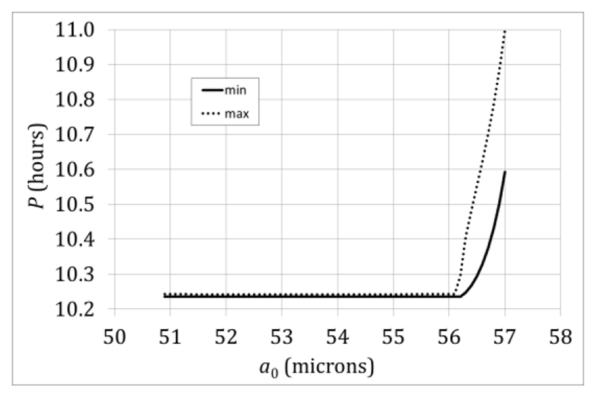
Figure 27
Profiles of pseudo-periods between minima (Pmin) and maxima (Pmax) estimated with Eq. (53), as functions of crystal half-width a0 (zw0 = 9 km).
Likewise, from the abscissae at the first three minima (xmin1, xmin2, xmin3) and maxima (xmax1, xmax2, xmax3) we can calculate two estimates Λmin and Λmax of wavelength by the formulae:
and plot the results as functions of a0 (Figure 28). The two curves have a bump in the range 51–56 μm with a maximum in the middle at a0 = 53.5 μm and they are separated by a gap of about 143 m, and a more exact value would be obtained from the transit through the asymptotic height z∞ calculated a posteriori from zmin and zmax (see below). These results are consistent with the value found in Sect. 3.2.3.
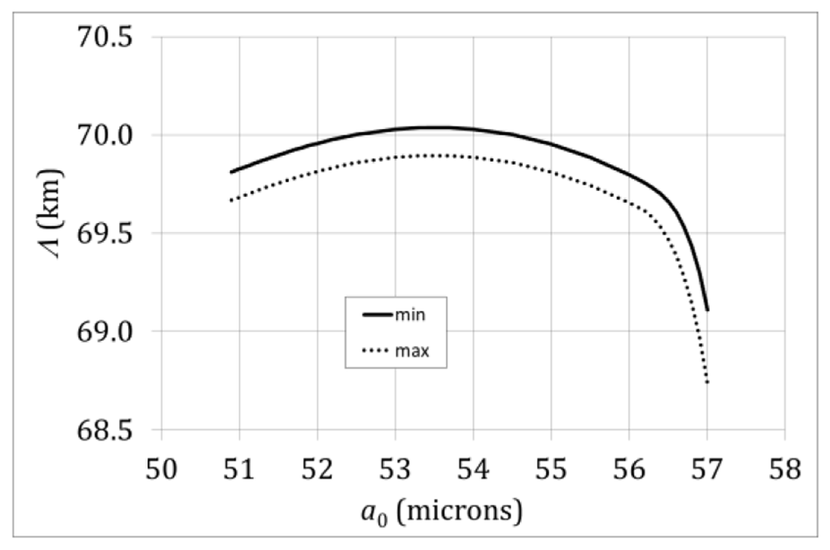
Figure 28
Profiles of wavelengths Λmin and Λmax derived from distances of minima and maxima by Eq. (54) as functions of crystal half-width a0 (zw0 = 9 km).
From periods and wavelengths, we can calculate corresponding phase speeds by Eq. (48), such that:
and plot the results as functions of a0 (Figure 29). Consistently with the variations of periods and wavelengths, phase speeds show a slow variation in the range 51–56 μm and they are separated by a small gap, Cmin and Cmax having both a maximum at the critical size a0 ≈ 53.5 μm.
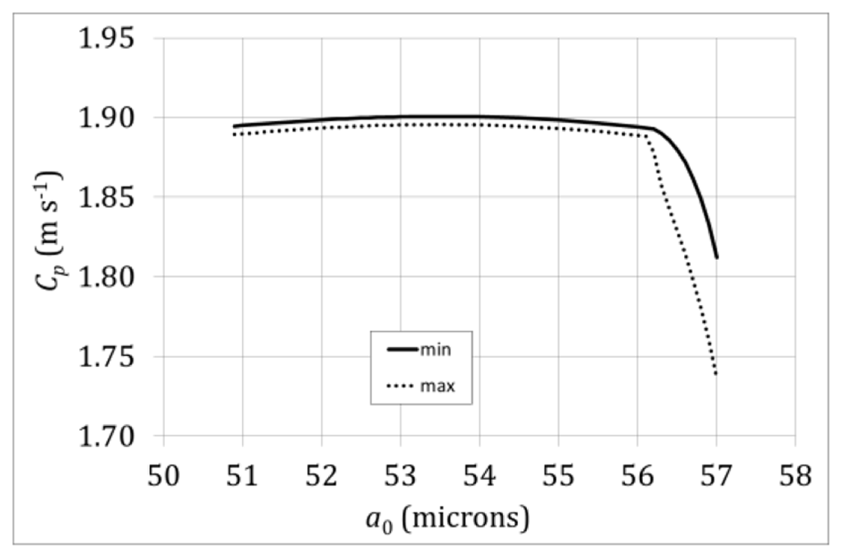
Figure 29
Profiles of phase speeds Cpmin and Cpmax derived by Eq. (55) as functions of crystal half-width a0 (zw0 = 9 km).
In contrast, plots of the altitudes at the minima (Figure 30a) and maxima (Figure 30b) reveal that their spacing depends on the crystal size and has a minimum at a0 ≈ 53.3 μm, corresponding to the size for which the formation of a hooked head is cancelled (Figure 25b).
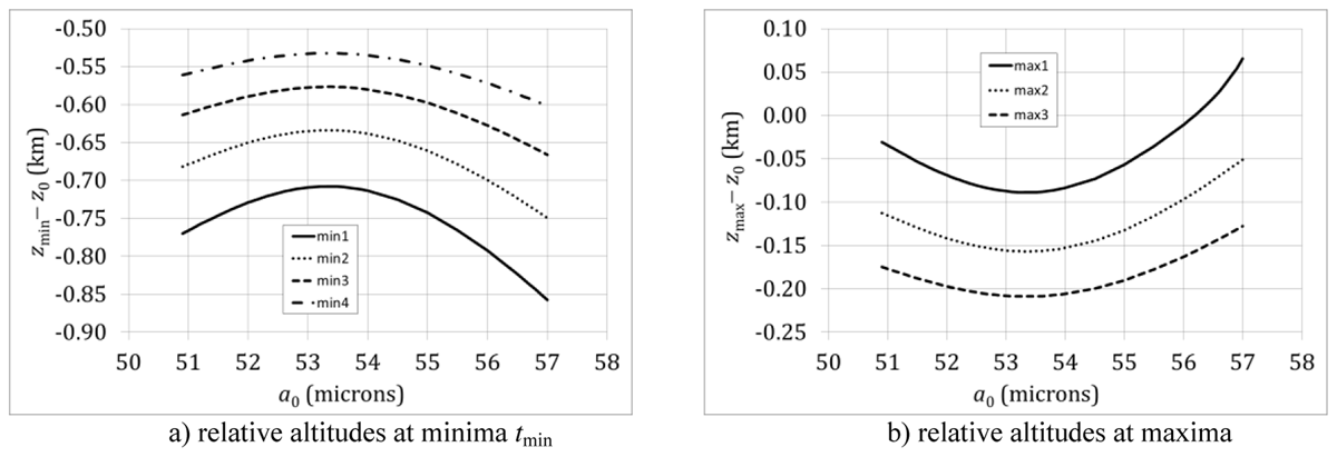
Figure 30
Profiles of relative altitudes at minima and maxima in the trail as functions of crystal half-width a0 (zw0 = 9 km).
Then, from the first three minima and maxima we can obtain a rough estimate of the limit height z∞ by the formula:
then we derive the limit velocity Ua(z∞) using Eqs. (68) in layer III: Ua(z∞) = –30 –5(z∞–16), and finally plot the results as functions of a0 (Figure 31). They show nice parabolic profiles within 1% in the range 51–56 μm of size, and again an extremum at a0 ≈ 53.3 μm.
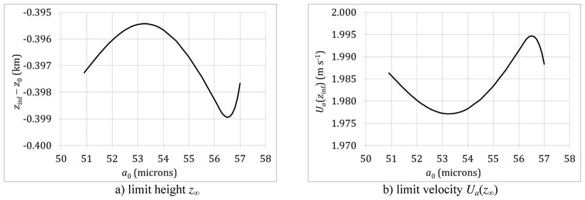
Figure 31
Profiles of relative limit height z∞–z0 and velocity Ua(z∞) in the trail as functions of crystal size a0 (zw0 = 9 km).
The damping ratio ζ appearing in the theoretical model of damped harmonic oscillator (App. D.2) can be estimated from our simulation data using the following procedure. The minimum and maximum altitudes can be written, within the approximation Ω ≈ Ω0:
Therefore, extracting ζ we obtain, for instance between extrema 1 and 2:
With the above data providing an average angular frequency Ω0 = 2π/(10.24 × 3600) = 1.7 × 10⁻⁴ rad s–1, and using an initial phase shift Φ ≈ π/4 (see App. D2), we obtain the value ζ ≈ 0.019, which is underestimated compared with the theoretical estimate of App. D.2 (ζ ≈ 0.05).
5. Impact of radiative transfer
5.1. Data
Although at temperatures as low as –50°C, ice supersaturation in observed cirrus clouds as large as 50% may be measured (Korolev & Isaac 2006), statistical data (Krämer at al. 2009) show average values equally distributed slightly above 0%, a situation that seems necessary to trigger damped oscillations when other conditions are favourable, but this is actually linked to the smallness of the radiative contribution. Thus, we shall show below that on one hand damped oscillations can develop with zero net radiative transfer (Case 1), and on the other hand we exhibit situations in which ice supersaturation is higher than in the standard case (Case 0) of Sect. 3.2.3 but associated with a higher net radiative transfer (Cases 2 and 3). The parameters and initial conditions are summarized in Table 2.
We shall display only the oscillatory mode and, following the same analysis procedure as in Sect. 3, we shall estimate period and wavelength as functions of the nominal water saturation, namely Ha3 at the latitude zH3 = 10 km, Eqs. (79) in App. A.3, and the radiative transfer ratio η which will be kept constant in this section. For each case, we show the trajectory, hodograph, and altitude time profile which are sufficient to determine period P, wavelength Λ, and also ice supersaturation Si–1, radiative correction R, and driving factor Si–1–R. The maximum height of the initial hooked cap, zmax0–z0, and the limit altitude of the oscillatory motion, z∞, are also recorded in Table 2.
5.2. Case 1
We assume that η = 1, i.e. the net radiative transfer is zero (Table 2). This is therefore a neutral case from a radiative standpoint. We choose the growth mode such that ϕ = 2 and cB is constant. With a radius a0 = 50.17 μm, steady and oscillatory modes are obtained just by switching the updraft base altitude, with lifetimes of 5 hours and 40 hours respectively. For small saturations (Ha3 = 61%, Si ≈ 103%), an oscillation is triggered and slowly damped, much alike the standard case (Sect. 3.2.3). It is noteworthy that the maxima along the trajectory (Figure 32a) are sharp at the beginning and tend to become blunter and blunter, while the minima have nice round shapes all along the motion, like other parameters displayed below (z, Si–1). The initial amplitude of height oscillations is approximately 400 m, like in Case 0, and the oscillation pattern during 40 hours spans a little more than 250 km (Figure 32a).
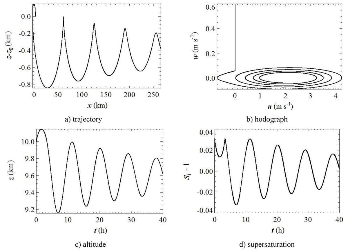
Figure 32
Profiles of the parcel trajectory, hodograph, altitude, supersaturation (η = 1; Wa = 0.6 m/s; Ha3 = 61%; zw0 = 9 km).
The maximum height reached in the head is 144 m, and then oscillation sets in, going through four maxima and four minima with moderate damping looking like the standard solution (Case 0) of Sect. 3.2.3. The period and wavelength derived from simulation results are approximately P ≈ 8.87 hours and Λ ≈ 64.8 km, which yield a phase speed Cp = 2.03 m s–1. The damping ratio is ζ ≈ 0.015. As expected, it is consistent both with the velocity limit u∞ ≈ 2.1 m s–1 in the slowly spiralling hodograph (Figure 32b) and with the wind speed at the limit height z∞ ≈ 9.58 km (Figure 32c), that is using Eq. (68) in layer III: Ua(z∞) = –30 –5(9.58–16) = 2.1 m s–1. The altitude time profile (Figure 32c) is qualitatively well described by the theoretical model of damped harmonic oscillator built in App. D.2 with moderate damping (Figure 41a).
Ice supersaturation (Figure 33d) oscillates at the same period and in phase with altitude (Figure 32c). The amplitude is approximately 2.5 % at the beginning and it decreases afterwards, tending towards zero.
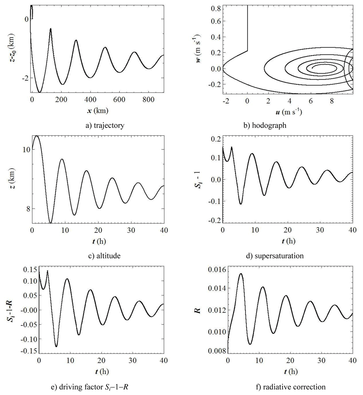
Figure 33
Profiles of the parcel trajectory, hodograph, altitude, supersaturation Si –1, driving factor Si –1–R and radiative correction R (η = 1.1; Wa = 0.8 m/s; Ha3 = 68%; zw0 = 7 km).
The absence of net radiative transfer results in a smaller period than in the standard case (Sect. 3.2.3), thus reflecting the property that the cloud lifetime is increased by radiative transfer (Dobbie & Jonas 2001). This can be called a dual case because the steady counterpart, not displayed, is characteristic of a well-developed cirrus uncinus.
5.3. Case 2
We assume here that η = 1.1, i.e. the net radiative transfer is positive and corresponds to higher layer in the upper troposphere where heating is predominant in daytime (Table 2). Therefore larger water and ice saturations (Ha3 = 68%, Si ≈ 115%), and updraft (Wa0 = 0.8 m s–1) are possible and the initial radiative correction can be larger (R ≈ 1.5 %) than in the standard case (R ≈ 0.8 %). Again choosing the growth mode such that ϕ = 2 and cB is constant, steady and oscillatory mode are obtained just by switching the updraft base altitude, with lifetimes of 4 hours and 40 hours respectively, upon specifying a radius a0 = 52.0 μm, and setting the updraft base altitude at 7 km, lower than in Cases 0 and 1.
The oscillatory mode is triggered again (Figure 33a), with a maximum height at 468 m in the cap followed by a trough at –2.5 km, then damped with wavelength Λ ≈ 200 km, period P ≈ 7.8 hours, and damping ratio ζ ≈ 0.02. According to Eq. (48), the phase speed is therefore Cp = 200 × 103 /(7.8 × 3600) ≈ 7.1 m s–1. As expected, it approximately matches both the focus u∞ ≈ 7.1 m s–1 of the quickly spiralling hodograph (Figure 33b) and the wind speed at the limit height z∞ ≈ 8.58 km (Figure 33c), that is using Eq. (68) in layer III: Ua(z∞) = –30 –5(8.58–16) = 7.1 m s–1.
The larger phase speed attained when the crystal parcel crosses the critical level (zU0 = 8 km) increases considerably the wavelength and consequently stretching beyond 900 km the span of the oscillation pattern during 40 hours (Figure 33a). The altitude time profile (Figure 33c) is in good agreement with the theoretical model of damped harmonic oscillator built in App. D.2 with the same period and a larger damping ratio (Figure 41b). Nevertheless, a significant period increase (≈ 7.5%) over 40 hours shows that the oscillator is not rigorously harmonic.
Ice supersaturation Si–1 (Figure 33d) oscillates at the same period and in phase with altitude (Figure 33c) like in the standard case (Case 0, Sect. 3.2.3). The amplitude of oscillations is approximately 15% at the beginning and it decreases quickly afterwards, as Si–1 tends towards the limit at 1.2% approximately. The radiative correction R (Figure 33f) is in phase quadrature with Si –1 whereas it was in phase in Case 0, and its limit is approximately 1.2%, equal to that of the supersaturation. Consistently, the growth driving factor Si –1–R (Figure 33e) oscillates about its limit, zero, with a large amplitude (≈ 10 %) at the beginning, larger than in Case 0 (≈ 2%), then quickly decreasing.
The hodograph (Figure 33b) shows an amazing feature consisting apparently in a folding of the spiral at the abscissa u = 10 m s–1 acting as a wall, a phenomenon that can be easily explained (App. D.2). This is well illustrated by the time profile of the horizontal velocity u (Figure 34), which clearly shows the first two eastward elongations truncated in the vicinity of Uamax. The subsequent elongations are not affected, and u eventually converges towards u∞ ≈ 7.1 m s–1.
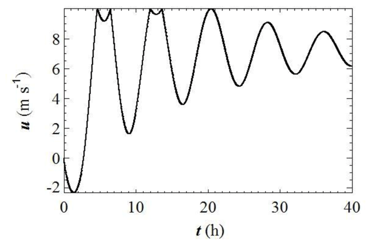
Figure 34
Time profile of the horizontal velocity u (η = 1.1; Wa = 0.8 m/s; Ha3 = 68%; zw0 = 7 km).
Like in Cases 0 and 1 before, the present damping ratio (ζ ≈ 0.02) is also underestimated compared with the theoretical estimate of App. D.2 (ζ ≈ 0.07). This case can be considered as isolated because the steady counterpart (not shown) is short (≈ 4 hours) and composed of a stretched hooked cap (≈ 20 km), without trail.
5.4. Case 3
We now assume that η = 0.9, i.e. the net radiative transfer is negative and corresponds to lower layers in the upper troposphere where cooling is predominant at night time (Table 2). Note that this is the particular radiative situation depicted by Eq. (25) in Sect. 2.2.2. Other parameters are set to values of the previous case (Ha3 = 68%, Si ≈ 115%, Wa0 = 0.8 m s–1; ϕ = 2; cB = cB0). Steady and oscillatory modes are obtained with lifetimes of 4 hours and 40 hours respectively, upon specifying a radius a0 = 53.9 μm, and setting the updraft base altitude at 7 km, lower than in Cases 0 and 1. The initial amplitude of altitude oscillations is approximately 1 km, and it decreases slowly afterwards (Figure 35a, c).
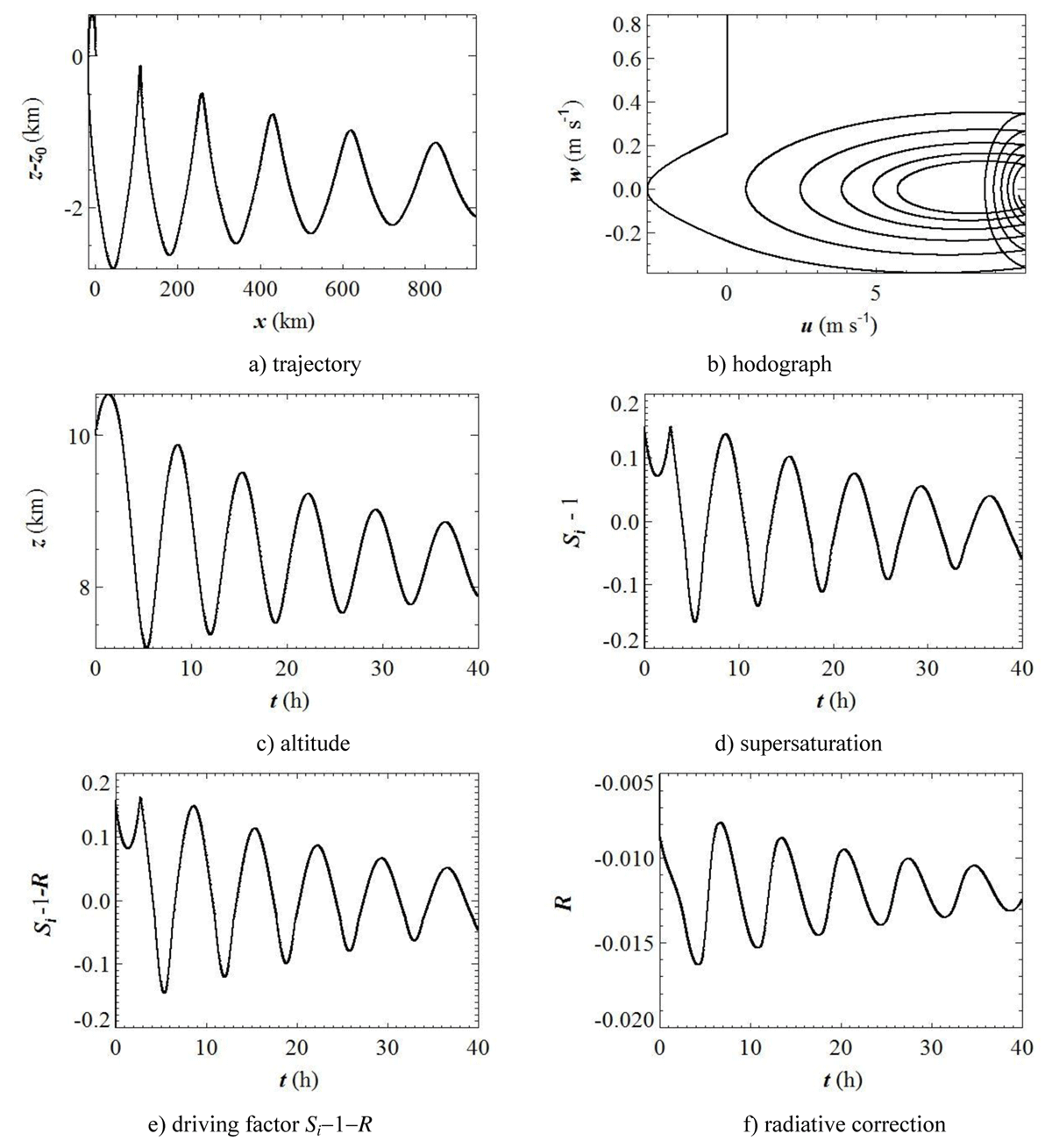
Figure 35
Profiles of the parcel trajectory, hodograph, altitude, supersaturation Si –1, driving factor Si –1–R and radiative correction R (η = 0.9; Wa = 0.8 m/s; Ha3 = 68%; zw0 = 7 km).
Thus the oscillatory mode is slowly damped with average Λ ≈ 200 km, P ≈ 6.8 hours, and ζ ≈ 0.01. According to Eq. (48), the phase speed is therefore Cp = 200 × 103/(6.8 × 3600) = 8.2 m s–1. As expected, it matches approximately both the limit u∞ ≈ 8.5 m s–1 in the hodograph (Figure 35b) and the wind speed at the limit height z∞ ≈ 8.3 km (Figure 23c), that is using Eq. (68) in layer III: Ua(z∞) = –30 –5(8.3–16) = 8.5 m s–1 Like in the previous case, the motion crossing the critical level (zU0 = 8 km) of maximum wind speed (Uamax = 10 m s–1) induces larger phase speed and wavelength, which causes the oscillation pattern during 40 hours to span more than 900 km (Figure 35a).
Ice supersaturation Si–1 (Figure 35d) oscillates at the same period and in phase with altitude (Figure 35c) like in other cases. Its amplitude is approximately 15% at the beginning and it decreases afterwards, as Si–1 tends towards the limit –1.2% approximately, slightly below saturation. The radiative correction R (Figure 35f) is again in phase quadrature with Si –1, whereas it was in phase in Case 0, and its limit is close to –1.2%. Consistently, the driving factor Si –1–R (Figure 35e) oscillates about zero, with a large amplitude (≈ 15 %) at the beginning, and as expected it tends towards zero.
We notice that the common limit of Si-1 and R at infinity are equal in magnitude but opposite in Cases 2 and 3 (R = ± 1.2%), a situation corresponding to opposite radiative initial conditions (η – 1 = ± 0.1). Moreover, the period shape in R oscillation is slightly asymmetric, the ascending half-period being steeper than the descending one in Case 3 (Figure 35f) and reciprocally in Case 2 (Figure 33f).
The hodograph (Figure 35b) shows here again a folding of the spiral at the abscissa u = 10 m s–1, but for five complete periods. The phenomenon, explained in App. D.2, is illustrated by the time profile of the horizontal velocity u (Figure 36), which clearly shows that all of the eastward elongations are truncated and folded in the vicinity of Uamax.
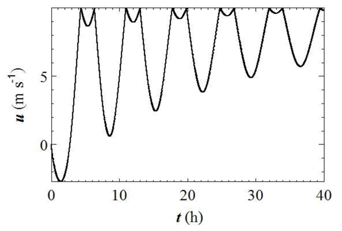
Figure 36
Time profile of the horizontal velocity u (η = 0.9; Wa = 0.8 m/s; Ha3 = 68%; zw0 = 7 km).
This case can be considered as isolated because the steady counterpart (not shown) is shorter (4 hours) and composed of a hooked cap with a horizontal extension of 20 km, without trail. The comparison of estimated damping ratios ζ (Table 2) reveals that Case 2 is more damped than Case 3.
6. Discussion
6.1. Non-oscillatory mode
Early simple analytical models of cirrus produced parabolic or quasi-parabolic shapes (Ludlam 1948; Marshall 1953). Among a lot of works on cirrus uncinus clouds supported by field observations, two series of papers using a Lagrangian approach, the first one published in the sixties (Magono et al. 1967; Yagi et al. 1968; Harimaya 1968; Yagi 1969) and the second one in the seventies (Heymsfield 1973; Heymsfield 1975a; Heymsfield 1975b; Heymsfield 1975c) retained our attention.
The first series reports stereoscopic observations that show real motions to be three-dimensional, the cirrus uncinus being also bent in a horizontal plane (Magono et al. 1967; Yagi et al. 1968; Harimaya 1968; Yagi 1969). The directions of cloud and wind are slightly tilted by 10° or so at the top of the trail and they are practically coincident at the bottom (Yagi et al. 1968).
The simple model based on these observations (Harimaya 1968) solves the mass growth equation Eq. (10) for crystal size and inserts the result in an analytic expression for the falling velocity, which in turn is integrated to yield the height as a function of time. Likewise, abscissa is obtained by integration of the horizontal drift velocity. Six crystal shapes are investigated and the wind shear is chosen in the range 0–7 × 10⁻³ s–1. Consistently with our result, the maximum fall speed of 0.5 m s–1 is reached 500 m below the origin. Nevertheless, temperature and humidity are assumed constant during the motion and, in the absence of updraft, no hooked cap is retrieved at the root of the trail. The cap is supposed to form within a turbulent layer between two stable layers (Yagi 1969).
The second series investigates the trajectory of five classes of crystals of bullet-rosette type, mostly observed in cirrostratus clouds (Heymsfield 1973; Heymsfield 1975a). By numerical integration of ODE analogous to our Eqs. (42), (43), (44) over a shorter time (3000 s), with an updraft velocity of 1 m s–1, characteristic shapes with a hooked head and a trail are retrieved. The major differences with our work lie in the facts that the buoyancy force and effect of latent heat release are included in the entrainment vertical velocity Wa, that radiative effects are not taken into account and that the crystal habit is more complex and it is based on a mass-size relationship. As a consequence, the vertical extent of the head is somewhat larger, reaching 500 m.
6.2. Oscillatory mode
The response of atmospheric layers to a Kelvin-Helmholtz instability is an important issue that may produce wavy patterns in the upper troposphere (billow clouds; cirrus fluctus). This phenomenon is usually discussed by means of the Richardson number Ri, defined by the expressions (Lynch et al. 2002):
with the Brunt-Väisälä angular frequencies ΩBVd and ΩBe, defined by (Durran & Klemp 1982):
and ΩBVm in a moist atmosphere, defined by (Durran & Klemp 1982):
and the horizontal wind shear ω:
The dry and equivalent potential temperatures θd and θe are usually defined by (Durran & Klemp 1982):
Vertical profiles of the local Richardson number (Figure 37) obtained with our data (App. A) show that the minimum value, reached at the inversion altitude of 8 km is approximately 2.95 in the dry case (solid line), and since it is everywhere larger than the critical value 0.25, we can conclude according to the criterion that the dry atmosphere is stable (Lynch et al., 2002). In contrast, the moist and equivalent profiles (dotted and dashed lines), which are not very different from each other, clearly show that a Kelvin-Helmholtz instability is likely to occur locally in such an atmosphere above and below 7 km, since Rim < 0.25. Published profiles show the same behaviour (Wada et al. 2005; Spichtinger 2014). Other authors (Dobbie & Jonas 2001) derived a radiative stability number Rsn and a criterion for onset of convective instability as: 0 < Rsn < 1. With a typical heating rate K d–1 at the altitude z = 9 km, they show that their criterion could be satisfied.
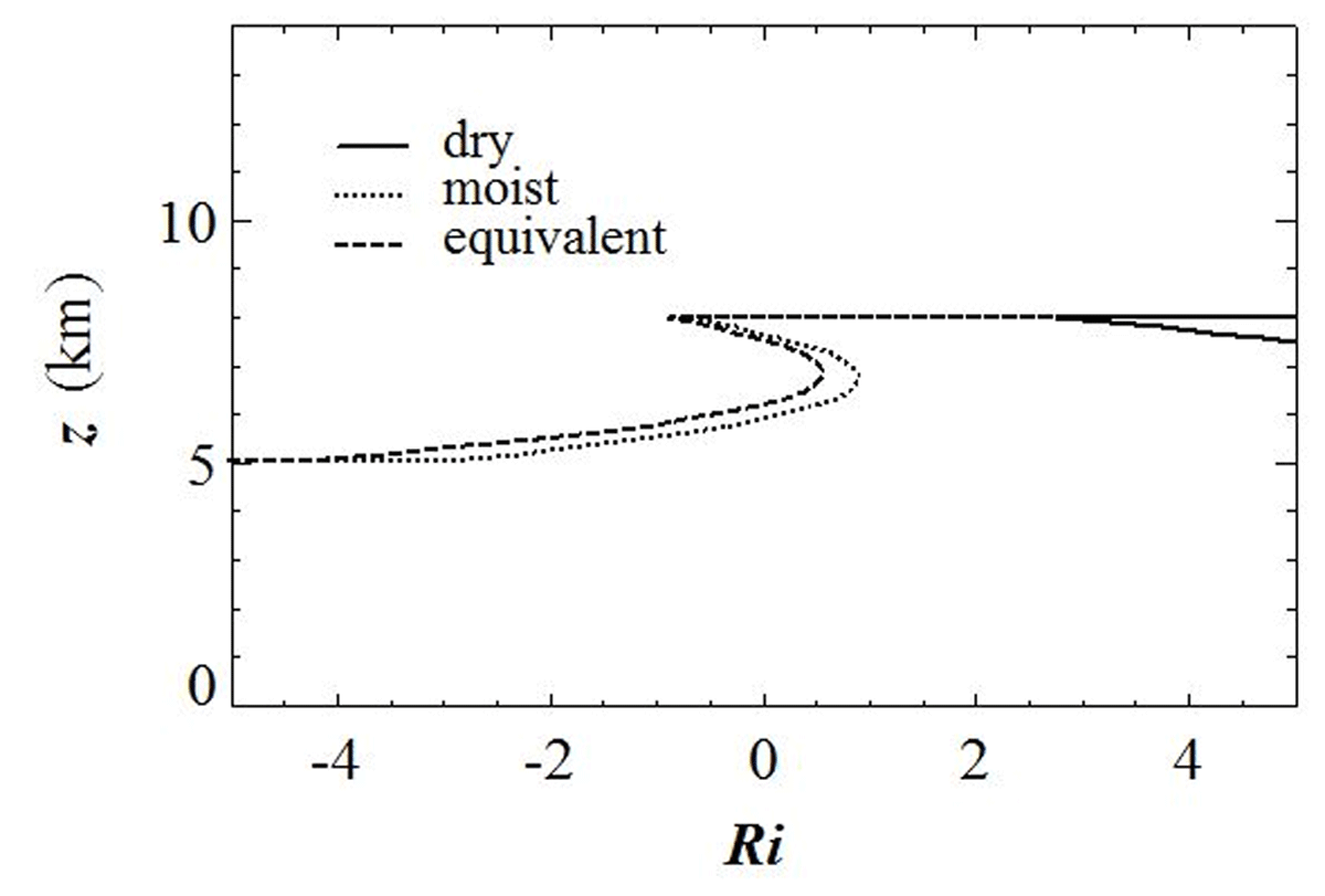
Figure 37
Atmospheric profiles of Richardson numbers.
In contrast, the oscillations we have put into evidence in Sect. 3.2.3 are due to the interplay of the crystal’s mass variation by deposition-evaporation and the updraft, and therefore it is neither a buoyancy effect relevant of Kelvin-Helmholtz instability nor a radiative instability, though the above remarks clearly suggests that these kinds of instability may develop in the free atmosphere at the altitude where our cirrus develops, or slightly below. Moreover, we notice that the two kinds of motions we found are such that the life time of a well-developed cirrus uncinus in steady mode is of same order as the half-period of the associated oscillatory pattern.
These oscillations were not found in the quoted work (Heymsfield 1975b), but the mention of “long-lasting cirrus turrets” originating from the trail and produced either by convection above the stable layer or by evaporation of ice crystals and the reference to generators of pulsating-type strongly suggests that they may be related to such observations. Nevertheless, low to moderate ice supersaturation in the range 3–15% seems to be more favorable to the onset of oscillations in our situation, in agreement with statistical data (Krämer at al. 2009), though values as high as 50% could be expected at such low temperature of –50°C according to some other data (Korolev & Isaac 2006).
The parcels being generated continuously in the head and feeding the trail downstream, the phenomenon may also be connected to the more recent concept of “Mesoscale Uncinus Complex” (MUC) that was proposed to explain the grouping of individual cirrus uncinus so as to form mesoscale structures with dimensions ranging from 15 km to 100 km (Sassen et al. 1989), consistent with our long-wavelength oscillatory pattern. The idea of MUC was confirmed afterwards by a series of observations (Wang 2004; Wang & Sassen 2008). Nevertheless, the phase speed Cp we estimate is related to the wind velocity at the altitude of oscillations (Cp ≈ 2–8 m s–1) and it is much smaller than the wind speeds (Ua ≈ 30 m s–1) involved in MUC and related to jet stream (Wang & Sassen 2008).
A first investigation (Demoz et al. 1998) using wavelets to analyze observations of low cirrus uncinus culminating at 8 km, shows spatial scale features of 30 km in extension associated with relatively high frequencies (≈ 0.007 Hz), corresponding to periods of 140 s. As shown by our Figure 37, convective instability is likely to develop at the altitude of their observations, so that the authors logically conclude that the high frequency spectrum (slope –5/3) is due to turbulence, and the low frequency component (slope –3) is due to the interaction of convection with gravity waves.
Another wavelet analysis (Wang & Sassen 2008) focusing on a high-altitude MUC (10–13.5 km) also reveals that two superimposed spectral components emerge: a small-period one (10–100 s) in a small scale range (0.4–4 km) with slope –5/3 relevant of turbulence in embedded cells, and a large-period one (100–1000 s) in a large-scale range (5–10 km) with slope –3, not relevant of a uniquely identified dynamical phenomenon, but rather resulting of the complex interaction of propagating gravity wave through turbulent layers. These efforts show that the phenomenon deserves further investigations in a range of larger periods (> 1000 s).
7. Conclusion and prospects
7.1. Results and findings
According to our purpose, using a Lagrangian approach with prescribed wind and updraft, we could retrieve the two-dimensional shape as well as dynamical and microphysical features of crystals trajectories leading to a well-developed cirrus uncinus. Moreover, besides this “standard” steady mode shaping a cirrus cloud, we put into evidence a self-sustained, damped quasi-harmonic oscillatory mode of long period (≈ 6–10 hours) and wavelength (≈ 60–200 km), never reported before, as far as we know. Despite its apparent simplicity, our model includes many elementary nonlinear processes, and it shows how the height of the updraft base, and radiative transfer competing with supersaturation, by modulating water vapour-ice phase changes that drive the crystal’s mass variation, can significantly modify the development of a mean ice crystal parcel. Nevertheless, small to moderate ice supersaturations in the range 3–15% seem to be more favorable to the onset of oscillations than values as high as 50% that could be expected at such a low temperature of –50°C (Korolev & Isaac 2006). Of course, this an idealized picture that requires an updraft stable over several tens of kilometers in the upper troposphere.
The complexity of our two-dimensional model can be quantified by 43 degrees of freedom, composed of the 36 constants implied in the ambient vertical profile conditions (App. A): dynamics (Ua, Wa) and thermodynamics (Ta, pa, Ha, ηa), supplemented with the 7 initial scalar conditions: position (x0, z0), velocity (u0, w0), column half-width (a0), aspect ratio (ϕ), hollowness factor (ψ). Of the total, we matched only five of them: zw0, Wa0, Ha3, ηa and a0.
By a detailed sensitivity analysis (Sect. 4) we have shown that the crystal size has a significant impact on the head extension and decay duration of the steady mode, but a smaller impact on the period of the oscillatory mode. Moreover, we examined the influence of radiative transfer (Sect. 5) in three specific situations, showing in particular that heating has a larger damping effect than cooling. This variability is a useful structural input for the modelling of cloud texture, as imagined in the prospective section below.
We notice that the two kinds of motions we found are such that the life time of a well-developed cirrus uncinus in steady mode (≈ 5 hours) is of same order as the half-period of the associated oscillatory mode (≈ 8–10 hours). An analytic model in App. D. recovers the computed shapes of the two modes and expressions of the period and damping ratio of the oscillatory mode are derived. A slight asymmetry of oscillations and a significant increase (≈ 7.5%) of period with time reveal some inharmonicity of the oscillator when radiative transfer is of constant sign, either positive i.e. heating (Sect. 5.3) or negative i.e. cooling (Sect. 5.4).
The theoretical background of the underlying Liénard differential system governing our system, which produces bifurcations due to a particular parameter (level of updraft base), is linked with the notion of strange attractor, actually originated in the astrophysical modelling of the dynamo effect maintaining stellar and planetary magnetic fields (Rikitake 1958), although roots are found in the modelling of population dynamics (Verhulst 1838; Vogels et al. 1975). Thus, the phase shift between the oscillations of mass and supersaturation that we put into evidence (Sect. 3.2.3) is quite similar to that appearing in predator-prey models (Koren & Feingold 2011).
In clouds, conceptual one-dimensional models (Wacker 2006; Spreitzer et al. 2017) have shown the importance of stratification and updraft in the interaction between a two-layer cloud system, and how time oscillations are generated according to the choice of parameters. Nevertheless, the periods are much shorter (15 to 50 minutes in the first model, 1.5 hours in the second) than those exhibited in our problem (6 to 10 hours), and the lifetime of the cirrus uncinus.
The possible connection of our theoretical model with the concept of Mesoscale Uncinus Complex (MUC) (Sassen et al. 1989) and periodic generating cells or ascending turrets (Heymsfield 1973; Heymsfield 1975b, 1975c) that we mentioned in the discussion (Sect. 6.2) would be a valuable application that deserves further investigations, looking for cells of several tens of kilometers pulsating over periods of several hours.
Assuming no motion along y coordinate, we also neglected the three-dimensional development of the cloud (see App. A3). Actually, radar and lidar observations usually provide mappings in vertical planes (Hogan & Kew 2005; Wada et al. 2005). At extremely low temperatures (T – Tr ≤ –50°C) we reasonably neglected liquid water in the cloud (Cziczo et al. 2013).
7.2. Prospects
As mentioned in Sect. 2.2.3, apart from single column, bullet-rosette is the most common crystal shape in cirrus uncinus (Heymsfield & Iaquinta 2000; Schmitt & Heymsfield 2007) and therefore we could also consider bullet-rosettes instead of hollow columns. The relevant parameters governing the growth are initial mass, capacitance, ventilation coefficient and drag coefficient. Mass will be roughly multiplied by the number N of bullets: m = N mb, and, instead of Eq. (41), the capacitance could be modelled as (Chiruta & Wang 2003):
In a first step, a simple 4-bullet rosette of plane type 4–4 (Heymsfield and Iaquinta 2000; Westbrook et al. 2008) could be used. Therefore, assuming bullets similar to our hollow column except for the ends, mass would be approximately multiplied by 4, and we would obtain C/a = 0.62, instead of C/a = 1.7, as shown from our Table 2. In other words, the crystal capacitance would be divided by 3 approximately.
Instead of Eq. (16) for a hollow column, the ventilation coefficient fv for broad-branch crystals and 1 < Re < 120 is given by (Ji & Wang 1999):
In our problem X ≈ 1.5 and fv = 1.4. A factor 2 on the size would increase Re likewise and consequently would multiply X by 1.4. Now, using (65), we would obtain: fv = 1.2, and this would probably not have a significant impact on crystal growth.
So far, the drag coefficient for bullet-rosettes seems to be an open concern, subject to constant investigations dealing with non-spherical particles and free-falling snowflakes (Heymsfield 1972; Haider & Levenspiel 1989; Heymsfield & Westbrook 2010; Vazquez-Martin et al. 2021; Aguilar et al. 2022). These approaches introduce the concepts of sphericity, projected area and Best number.
With 3 degrees of freedom (a, c, cB) or (a, ϕ, ψ) for each bullet, we could assume that all of the bullets grow at the same rate, with the same rules as for a single column. Nevertheless, it is known that the equilibrium shape of the crystal at each time should be calculated so as to minimize the total surface energy for a given volume (Pruppacher & Klett 1978). Moreover, at larger supersaturations, the capacitance model based on Eq. (10) presents limitations, that have been discussed by introducing the concept of impedance (Peter and Baker 1996; Nelson & Baker 1996). Alternative models of growth-evaporation based on this concept such as the TLK (terrace-ledge-kink) model have been proposed and applied to hexagonal ice crystals (Wood, Nelson, & Calhoun, 2001).
The vertical shear of the wind Ua and the base of the updraft Wa are essential input of our dynamical conditions, in order to produce the characteristic hooked shape of cirrus uncinus. The profiles of temperature and humidity are suggested by actual measurements in the troposphere but they may be varied. The trajectory is also very sensitive to the initial conditions, which may cancel the formation of a hooked cap.
Especially the wind field Ua we imposed throughout the present work has been chosen realistically according to published works (Kew 2003; Mace et al. 2005), but there is no standard profile for it, so that its minimum and maximum velocities could be varied in Eqs. (68) (App. A1), thus impacting the wavelength Λ of the crystal’s oscillation. Actually, the period P being an intrinsic property of the phenomenon, the wavelength can be derived from it via the phase speed Cp defined by Eq. (48), which is equal to the wind speed at the limit height z∞:
Thus, increasing or decreasing Ua in the layer under concern (III) will increase or decrease Λ accordingly. This gives some flexibility to the scale of our phenomenon, if it can be related to MUC (Sassen et al. 1989) and pulsating-type generators (Heymsfield 1973, 1975b, 1975c). In our situation, fast winds exist in layers (IV) above the layer of interest (III), but the wind shear we adopted, in agreement with published data, makes wind slower at the altitude where we produce the uncinus head, that could not arise otherwise.
Whereas Coriolis force can be neglected in the non-oscillatory mode, it may be included in a more accurate model of the oscillatory mode, since the extension of the structure over several hundreds of kilometers tends to the synoptic scale and may not be completely negligible compared to the Earth’s dimensions. Although the crystal’s motion is driven mainly by gravity and steady winds, atmospheric turbulence would add random degrees of freedom, and so contribute to the wispy appearance of cirrus. The governing system Eq. (1) would be modified as follows:
In the assembly of crystals forming a parcel, collisions between particles inevitably produce mechanical interactions, aggregation, and also electric interactions via the electric charges that are formed.
Moreover, the influence of atmospheric waves on the evolution of cirrus (Lin et al. 1998; Podglajen et al. 2018; Prasad et al. 2019; Kärcher et al. 2019) is a matter of concern, since it is invoked in MUC. Though they are not the driving mechanism of the oscillatory mode we found, as shown in Sect. 6.2, Kelvin-Helmholtz waves may develop at the altitude of 7 km or above. In a more elaborate model, these additional effects could be included in the modelling equations (67), and they would probably smear the motions about the two basic behaviours reported in the present work.
From an experimental viewpoint, observations would be welcome for investigating the intermediary spatial range between meso- and synoptic scale (300–1000 km), and longer time periods (>1000s) where the damped oscillations we numerically exhibited could be hopefully detected, in connection with MUC or ascending turrets. From a theoretical viewpoint, approximate analytical solutions of the differential system of Liénard-type governing the crystal’s evolution should be searched in order to derive more accurate expressions of the angular frequency Ω and the damping ratio ζ of underdamped oscillatory solutions, for which a demonstration has been sketched in App. D.2.
Extending the sensitivity analysis of Sect. 4 to an assembly of crystals of different sizes in a parcel and assuming particle densities would make possible the modelling of size distributions (Heymsfield, Schmitt, & Bansemer, 2013) and consequently the calculation of ice water content (IWC). Actually, apart from the understanding of natural phenomena, the generation of realistic cloudy scenes with radiative transfer is another valuable extension of the present work. In that purpose, we can imagine applying a textured IWC in the spatial and temporal frame elaborated herein, using spectral or fractal methods and the dynamic-microphysical output of our model. Such an approach has been intensively implemented for years to render various types of clouds, from stratocumulus and cumulus to cirrus (Cianciolo 1993; Evans & Wiscombe 2004; Hogan & Kew 2005; Sölch & Kärcher 2010; Szczap et al. 2014). In the case of liquid water clouds, a model of water content was widely used in cloud generators (Feddes 1974).
We also used such methods for stratocumulus (Berton 2008). Nevertheless, it seems that the approach should be different for stratocumulus and in-situ cirrus clouds: while the former are essentially due to convection, the latter evolve under a combination of advection and free fall. This issue has been considered in recent models (Hogan & Kew, 2005 Sölch & Kärcher 2010; Szczap et al. 2014) from a macrophysical point of view in order to render fall streaks.
Moreover, the very nature of the cloud particles –droplets in the former case, ice crystals in the second one – suggests that the medium, owing to the shape and orientation of crystals (Hashino et al. 2014; Hashino et al. 2016), is strongly anisotropic in the second situation. In that respect, a set of differential equations for the angular momentum could supplement the system of Eqs. (67), including the torques caused by fluid friction and the fact that the column is hollow.
The present approach enables the generation of horizontal inhomogeneities related to the history of ice particles along the trajectory, and this point is most important since these are known to be an important input in the modelling of radiative properties of cirrus clouds (Liou & Rao 1996; Buschmann et al. 2022; Kew 2003; Kokhanovsky 2003; Fauchez et al. 2014). Up to now, a few methods have been devised to remedy this problem (Shonk & Hogan 2008).
Appendix A. Atmospheric profiles
A.1. Atmospheric motions
The imposed atmospheric motions are composed of a uniform horizontal wind Ua with a given vertical profile (Figure 1), and a constant vertical updraft Wa, operating only above a critical level zw0 equal to either 10 km, 9 km, or 7 km (Figure 2). We built our horizontal wind profiles from published data (Kew 2003; Mace et al. 2005). A two-dimensional mapping in a vertical plane of combined observational data (Wada et al. 2005) clearly shows such patterns.
The horizontal wind profile we chose reflects the horizontal shear and the vertical convection necessary for the formation of the virga. The vertical profile of horizontal wind Ua(z) (Figure 1) is given as a piecewise linear function composed of four segments:
with the following 6 constants:
It is noteworthy that, with this choice of constants, Ua vanishes above the ground at the altitude z0 = 10 km. Moreover, the resulting wind shear ω, respectively equal to 1.0, 1.3 and –5 m s–1 km–1 in the ranges 0–5, 5–8 and 8–16 km, is quite consistent with observational data (|ω| < 23 ms–1 km–1) (Heymsfield 1975b; Heymsfield 1975c; Wada et al. 2005). As we show in section 3.2, the results are especially sensitive to zw0.
The updraft profile Wa(z) is chosen so as ensure that Wa is constant, non-zero above zw0 = 10 km (1st mode or regime) or zw0 = 7 or 9 km (2nd mode or regime) and zero below zw1 = zw0 – ∆z0, with a transition layer of thickness ∆z0 = 0.3 km, the transition profile being modelled by a linear function (Figure 2):
with the following constants:
We verify that such a two-dimensional flow satisfies the equation of mass conservation for air considered as an incompressible fluid:
Thus in the 300 m-thick transition layer, the gradient of updraft ∂Wa/∂z produces a shear of the horizontal wind ∂Ua/∂x in the x-direction equal to
that is smaller in magnitude than the vertical shear at the same altitude (ω = –5 m s–1 km–1). We notice that in a three-dimensional description of the motion, this shear may affect the perpendicular component of wind, Va, here set to zero, according to the complete equation:
and create a horizontal shear of Va in the y-direction. Now, things being as they are, since we assume that Ua is a function of z alone we shall neglect this horizontal shear of Ua compared to the vertical one, in solving the system (42).
A.2. Temperature and pressure
As suggested by measurements (Baum et al. 2000; Kew 2003), the vertical profile of temperature Ta(z) (Figure 3a) is given as a piecewise linear function composed of five segments:
with the following 10 constants:
while the pressure (Figure 3b) is given as an exponential function of height:
with the two constants: p0 = 101493 Pa and h = 7.5 km.
A.3. Humidity
Likewise, the vertical profile of relative humidity with respect to liquid vapour Ha(z) in the atmospheric clear sky (Figure 4a, solid line), as suggested by measurements in clear sky (Baum et al. 2000) and in an environment favorable to the generation of a cirrus cloud (Fusina and Spichtinger 2010), is given as a piecewise linear function composed of six segments:
with the following 12 constants:
On the same figure is then plotted (dotted line) the profile of Hi derived from Ha, first by calculating the water vapour pressure pv as solution of Eq. (84) below (Hl = Ha), then by estimating Si by Eq. (12b) and finally by deriving Hi by Eq. (13b). It is noticeable that Hi > Hl, as it can be easily proved from Eqs. (12) and (13), since pvsl > pvsi. We also plotted the profiles of Sl and Si (Figure 4b), though they are very close to those of Hl and Hi respectively. Moreover, the profiles of Hi and Si are plotted down to 2 km, altitude at which the temperature reaches the frozen point (Ta = 273.15 K). We notice that our profiles of Si are quite consistent with those of other simple models of cirrus uncinus (Harimaya 1968).
A.4. Radiative flux densities
Adopting Zeng’s parameterization (Zeng 2008; Zeng et al. 2021), we assume that the vertical profile of the radiative flux density in the infrared is described by the ratio ηa(z) defined by Eq. (23) and can be given in the upper troposphere as a piecewise linear function composed of three segments:
with the following 4 constants:
We lowered the altitude of the transition ηa = 1 because the original work (Zeng 2008) deals with tropical cirrus clouds while we are concerned with mid-latitude ones. The profile ηa(z) is plotted on Figure 5: the transition (ηa = 1) occurs at an altitude z = 9.5 km.
Appendix B. Calculation of the ambient pressure of water vapour
Since the ambient relative humidity Hl with respect to (wrt) liquid water is given (Hl = Ha), it is necessary to derive the pressure pv of water vapour by inversion of the relation (13a), with the total pressure such that:
we obtain the relation:
and after rearranging, a quadratic equation for pv can be finally written:
This equation has two real solutions because its discriminant δ is essentially positive:
Nevertheless, only the solution with + is physical, because it yields pv = pvsl as Hl → 1.
Appendix C. Saturation pressures of water vapour
According to Sonntag’s formulation, the saturation pressures of water vapour over liquid water and ice are respectively expressed as (Sonntag 1990; Alduchov & Eskridge 1996; Murphy & Koop 2005):
with the following coefficients:
Appendix D. Analytical model of trajectory
D.1. Non-oscillatory mode
Solving system (1) with analytic functions is a difficult task as soon as k and Wa are not constant. This is the object of Sect. 3, including the underlying microphysics. As an alternative, we consider here the non-oscillatory motion of an ice parcel subject to entrainment by horizontal wind Ua, constant and uniform vertical updraft Wa and free fall Wf, governed by the set of ODE:
with initial conditions (2). The single dot means first time-derivative. The horizontal wind is an approximation of the sheared flow in the range of altitude 8–12 km (Figure 1), with shear ω, which is cast into the linear form:
Therefore, the velocity Ua changes sign at the altitude zm such that:
Since the average crystal radius and mass decrease in the virga under the action of sublimation, the free fall speed Wf must also decrease as t tends towards infinity. We chose a unique analytical function Wf(t) defined in [0,+∞[, and satisfying the following conditions (Figure 38):
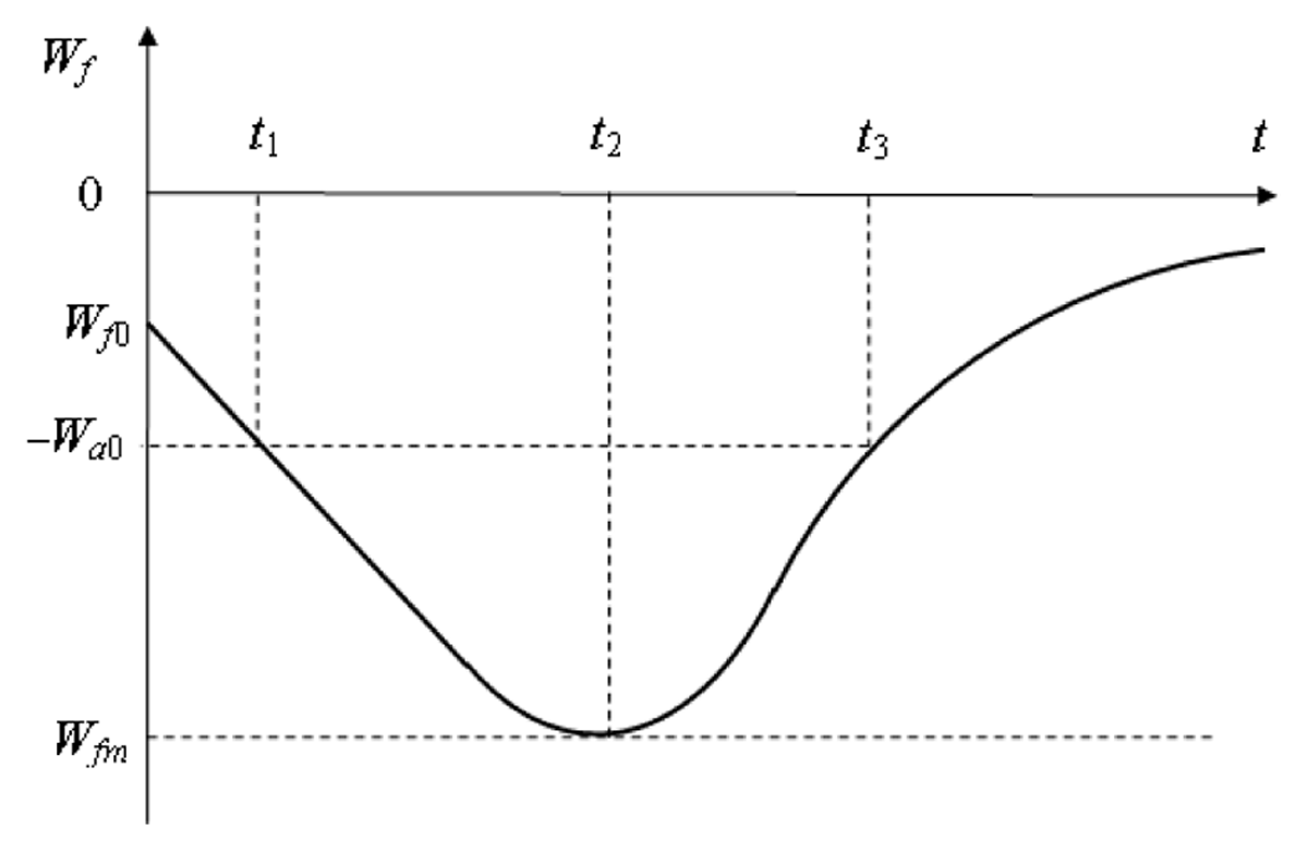
Figure 38
Qualitative time profile of analytical free fall speed.
Looking for a solution of the type:
that is subject to the conditions (91), we obtain the expression:
with the characteristic times t1 and t2 such that:
and:
The non-dimensional parameter τ is solution of the classical transcendental Lambert-type equation (Corless et al. 1996):
Substituting the expressions (89) and (93) in the dynamic system (88), we obtain at any time t Î[0,+∞[:
The integration of the system of first order ODE (97) subject to the following initial conditions:
yields the expressions for x and z:
Eqs. (99) are the parametric equations of a transcendental curve, more complex than the basic parabolic shape (Marshall 1953; Hogan & Kew 2005).
We can notice that the behaviour at infinite time, involving the secular terms in Eqs. (99), is not relevant since the variable-mass crystal eventually vanishes through sublimation and precipitation. Moreover, our model considers a flat Earth, an assumption which implies neglecting Coriolis force and focusing on the behaviour at local scale (less than 100 km).
A maximum occurs where , at a time tM that is again a solution of the transcendental Lambert-type equation (Corless et al., 1996):
of which tM = t1 is the solution in the principal branch. Likewise, an extremum occurs where , at a time tm solution of a complicated transcendental equation. In contrast, the altitude zm of the extremum is simply given by Eq. (90).
An example of motion was sampled at 601 points over a 6000-second life time (≈ 1.7 hour) with a time step ∆t = 10 s and the following values of parameters:
We choose the following value of wind shear: ω ≈ –5 × 10⁻³ s–1, consistently with published values (Harimaya 1968; Wada et al. 2005) which recommend: |ω| < 23 m s–1 km–1. Estimating the solutions of Eq. (96) and the zeros of the derivatives (97), we obtain the following characteristic times and passing times through extrema:
The non-dimensional parameters r and τ defined by relations (95) respectively take the values: r = –0.5 and τ = 0.232. The trajectory (Figure 39a) has a nice hooked-shape head expanding vertically between 0 and t1, like that obtained with the full model (Figure 7a). Nevertheless, the updraft Wa is constant in the whole atmosphere in the present analytical model, while it is zero below zw0 and nonzero above in the full model.
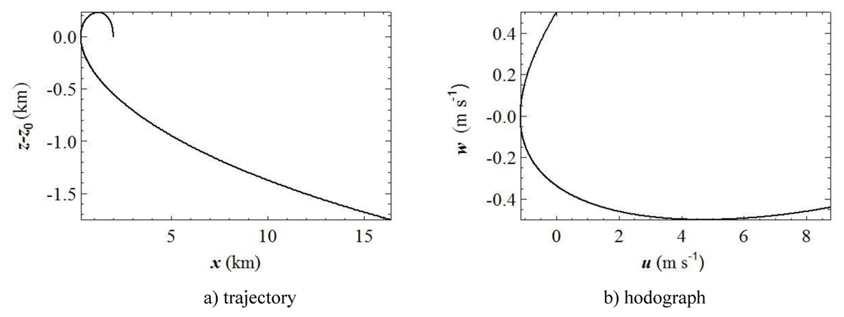
Figure 39
Trajectory and hodograph for analytic solution, Eq.(99).
The theoretical hodograph (Figure 39b) is qualitatively similar to that obtained with the fully coupled model (dynamics/microphysics) (Figure 7b). Likewise, the theoretical profile of free fall speed (Figure 40) is qualitatively similar to the assumed profile (Figure 38) and to that of the full model in non-oscillatory mode (Figure 9a).
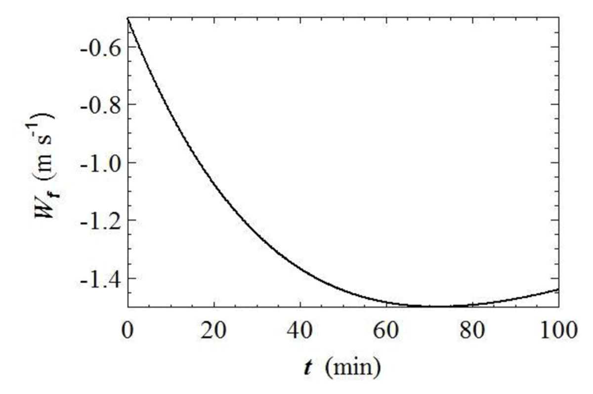
Figure 40
Time profile of free fall speed for analytic solution, Eq.(99).
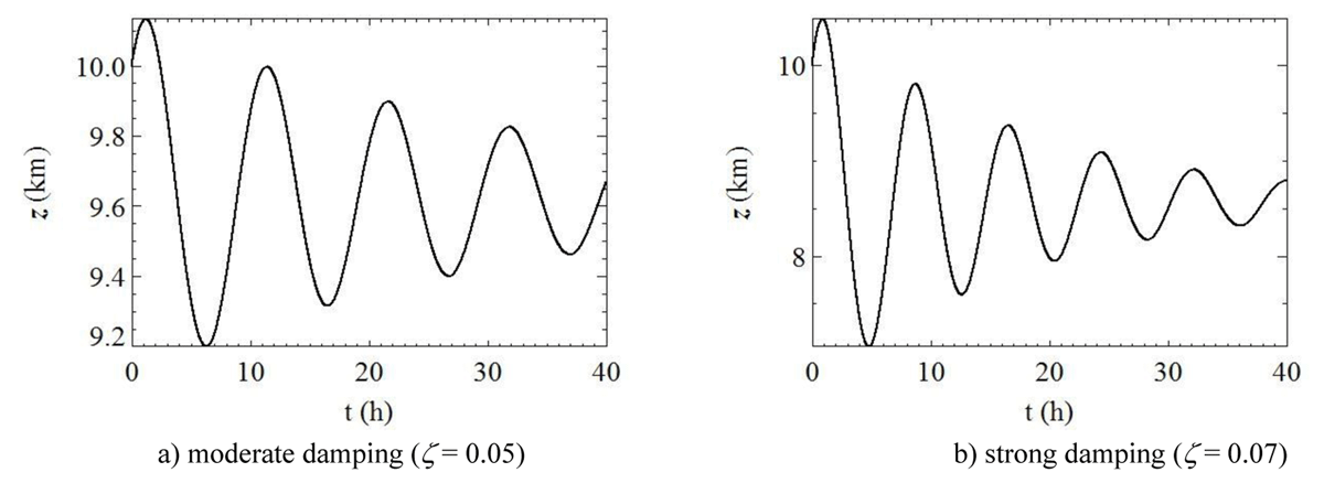
Figure 41
Altitude time profile of theoretical underdamped harmonic oscillator, Eq.(118) for moderate (a) and strong (b) damping.
Casting Eq. (10) as:
with ∆S denoting the factor Si–1–R, and integrating between t = 0 and t > 0 at approximately constant rate yields:
which yields an estimation of the crystal’s life duration tmax when m(tmax) vanishes:
With the following typical values obtained from simulations of Sect 3.2: m0 ≈ 10–9 kg, ≈ 2 × 10–12 kg s–1, ∆S ≈ – 0.02, we obtain: tmax ≈ 7 hours. This elementary calculation shows that a crystal falling through highly saturated layers with a large variation of the growth factor (|∆S| >> 0.1), combining the effect of ice saturation and radiative transfer, cannot be long-lived.
D.2. Oscillatory mode
1) Our purpose here is to derive a theoretical ODE proving the existence of damped oscillations as solution, and tentatively expressions of angular frequency and damping ratio. We first note that the full system:
is a system of second order ODE of Liénard-type of the general form:
that can be cast more explicitly into the form:
that is itself a set of coupled Abel equations of the second kind.
Now, neglecting the coupling with horizontal motion, we can thus write the equations of evolution of vertical motion and mass Eqs. (1b) and (10) in the form:
where single and double dots respectively mean first and second time-derivative, and the mass growth rates are defined by:
Then expanding Si–1 to first order in the vicinity of the equilibrium height z∞:
and noting that:
we derive a relation for the vertical mass gradient:
Likewise, let us expand the velocity in the vicinity of z∞:
and upon inserting this expression into Eq. (111) we obtain a simple ODE for mass:
which yields by integration over z between z0 and z:
Likewise, let us expand the effective radius ri in Eq. (108) after Eq. (38):
with the asymptotic equivalent diameter:
Substituting these expressions for mass and radius into Eqs. (107b) and (108b) and rearranging, we finally arrive at the fundamental ODE of a damped harmonic oscillator:
The second term represents the damping friction and the third one the restoring force producing the oscillation. Eq.(117) clearly shows that it is necessary that an updraft exists (Wa ≠ 0) below the generating height (z < z0) for a long-period oscillation to take place.
Satisfying the conditions at initial time (z = z0) and infinity (z = z∞), a solution of the homogeneous equation in the case of an underdamped oscillator can be written as (Meirovitch 1986):
with phase Φ ≠ 0. The angular frequency Ω0 and the damping ratio ζ are such that:
After substitution of mass growth rates, Eqs. (108), they can be written:
Using the following values derived from the simulations of Sect 3.2: m∞ ≈ 10–9 kg, μa ≈ 10–5 Pa s, C ≈ 10–4 m, ri ≈ 10–4 m, fv ≈ 1, σS ≈ 7 × 10⁻⁵ m–1, ω ≈ 5 × 10⁻⁵ s–1, we can estimate Ω0 and ζ as:
The angular frequency thus obtained is larger than the effective value obtained in Sect. 3.2.3 and 5.2, namely Ω0 ≈ 1.7 × 10⁻⁴ rad s–1, and the damping ratio, compared to ζ = 0.05, has also too large a value, that would characterize an overdamped oscillation. This large discrepancy is probably due to the fact that most variables of the problem are dependent of temperature, itself being altitude-dependent, especially in the mass equation (Eq. (10)), in the mass rates and (Eq. (108)) we assume constant. A full treatment would necessitate an expansion of all these variables as functions of temperature, and eventually use of Eqs. (75).
In order to illustrate the original behaviour we found in Sections 3 and 5, we plot time profiles of altitude as modelled by Eq. (118) with constants associated to “moderately” and “strongly” damped harmonic oscillators (Table 3). The resulting profiles (Figure 41) are visually matched with the corresponding profiles of numerical solutions, displayed respectively in Sect. 3.2.3 (Figure 17b) and Sect. 5.2 (Figure 32c) for moderate damping and Sect. 5.3 (Figure 33c) for strong damping. The agreement is very good except at the beginning of the motion because the time spent by the crystal in the hooked cap broadens the first period (t < 5 hours), so that the subsequent periods are slightly shifted to the right in the actual motion. Inharmonicity detected in numerical simulations probably enhances that effect and suggests to analyse it further with the method of Krylov and Bogoliubov (Bose et al. 1989).
Table 3
Parameters of theoretical periodic profiles.
| DAMPING | MODERATE | STRONG |
|---|---|---|
| z0 (km) | 10.0 | 10.0 |
| z∞ (km) | 9.63 | 8.58 |
| P (hour) | 10.2 | 7.8 |
| Ω0 (rad s–1) | 1.71 × 10⁻⁴ | 2.24 × 10⁻⁴ |
| ζ | 0.05 | 0.07 |
| Φ (rad) | π/4 | π/4 |
2) This short subsection is devoted to the explanation of foldings produced in the hodograph and horizontal velocity profiles of Cases 2 (Sect. 5.3) and 3 (Sect. 5.4). Let us recast the ODE governing horizontal velocity, Eq. (1a), as:
Since k is positive, Eq. (122) shows that when u > Ua, then and u decreases to Ua in a drag relaxation time τD = 1/k (Paoli & Shariff 2016), and reciprocally when u < Ua. Since τD is of order of time step ∆t, the relaxation is quasi instantaneous and therefore u follows the variation of Ua. Numerical experiments in Sect. 5 reveal that the difference u–Ua is of order 10–4 m s–1, so that with k ≈ 10 s–1, the crystal undergoes horizontal accelerations of order 10–3 m s–2. In the vicinity of the maximum wind speed Uamax, u is therefore constrained to remain smaller than Uamax, and thus u profiles (Figures 34 and 36) show two spikes per period, corresponding to the ascending and descending branches of Ua profile in the vicinity of Uamax = 10 m s–1 at the altitude of 8 km (Figure 1). The folded loops in hodographs are a result of that phenomenon.
Acknowledgements
The author is very grateful to the reviewer for important and insightful comments which contributed to greatly improve and enlarge the content and discussions of the article.
Competing Interests
The author has no competing interests to declare.