
1. Introduction
The sea ice cover is often used as an indicator of the global environmental change that modulates the albedo, ocean-atmospheric circulation, cryosphere ecosystems, and biogeochemical cycle. The underlying cause of the Antarctic sea ice variability triggered by the ocean-atmospheric processes has remained a crucial question both for the scientific community and policymakers. The global climate is changing and putting the globe on the verge of irrevocable change. Through 2015, the world has warmed by 0.87°C, relative to pre-industrial levels, as reported by the International Panel on Climate Change (IPCC, 2018). This temperature rise is attributed to the net increase in climate forcing due to the surge in atmospheric CO2 in the last 20 decades (Stips et al., 2016). The global temperature anomaly shows a continuously increasing trend since 1994, up to 1°C, with a sharp rise in the years 2016 and 2020, followed by the years 2017, 2019, and 2021 (Hansen et al. 2010). The concentration of CO2 in the Earth’s atmosphere has risen by a factor of 1.22 since 1980. The value of CO2 concentration in 1750 was 277 ppm, to 338.45 ppm in 1980 and upsurged to 418 ppm in 2022 (J.Conway et al., 1994; www.esrl.noaa.gov/gmd/ccgg/trends/).
The polar regions have encountered a more stunning transformation than most regions of the world. The sea ice variability in the Southern Ocean observed an overall expansion, along with the diverse patterns of advancing and retreating sea ice on a regional scale. The positive trend of sea ice was more pronounced between 2000 to 2014, nearly five times the growth observed between 1979 and 1999, to reach a record-high annual mean sea ice extent (SIE) of 13.18 × 10⁶ km2 in 2014 (Parkinson, 2019). The rapid sea ice growth is linked to a slowdown in the rate of global warming that occurred when the Interdecadal Pacific oscillation (IPO) was at its negative phase along with the contribution from convective heating anomalies in the South Pacific convergence zone (SPCZ) regions and the strengthened westerlies (Eayrs et al., 2019; Meehl et al., 2019). The IPO is a long-timescale index varying from 20-30 years and represents the oscillation of western Pacific temperatures similar to El-Niño. The negative phase of the IPO is responsible for the strengthening of the westerlies and Amundsen Sea Low (ASL) deepening, while the positive phase of IPO favors the weakening of westerlies and anomalous high pressure in ASL (Eayrs et al., 2021; Li et al., 2021). The positive sea surface temperature (SST) anomalies in the central Pacific and the southwest movement of SPCZ during IPO– triggered the poleward propagation of Rossby waves in all the seasons. These wave trains intensified the ASL through the consistent negative pressure anomalies in the region near Amundsen and Bellingshausen Seas (BAS) from 1999 to 2015 (Eayrs et al., 2021; Meehl et al., 2019). Also, the Atlantic Multidecadal Oscillation (AMO) represents the SST variability in tropical Atlantic affects the Antarctic atmospheric circulation through the propagation of Rossby waves (Li et al., 2021).
In the southern hemisphere, the advection of ozone depleting gases from anthropogenic sources into the Antarctic atmosphere caused stratosphere cooling during 1979–2015 (Meehl et al., 2019). This cooling increased the meridional temperature gradient which strengthened the polar vortex reinforcing the polar jet stream around the Antarctic. The increase in meridional pressure gradient (pole-equator) has led to an increasing trend of the southern annular mode (SAM) with the strengthening and poleward shifting of westerlies. These processes promoted the sea ice growth through enhanced northward advection of low-saline cold water from the coastal Antarctic. Also, the intensified westerlies associated with positive SAM act as a shield to prevent the intrusion of warm air in the Antarctic, thereby enhancing ice growth (Polvani and Smith, 2013; Thompson et al., 2011). The changes in both SAM and ASL are influenced by the large-scale atmospheric teleconnections linked to the occurrence of explosive polar storms (Francis et al., 2019) and tropical SST variability in the form of climate oscillators such as ENSO (Eayrs et al., 2021; Yuan, 2004), AMO (Atlantic Multidecadal Oscillation) (Li et al., 2021, 2014), and IPO (Meehl et al., 2019, 2016).
Several studies looked into the characteristics of meteorological and oceanic mechanisms linked to a dramatic loss of sea ice in 2017. The asymmetric component of the atmospheric circulation located in the higher latitudes of the southern hemisphere, represented dominantly by the zonal wave three (ZW3) and zonal wave one (ZW1), is responsible for meridional transport of heat and moistures (Raphael, 2004). The amplitude of the ZW3 pattern is determined by the temperature gradient variability, with a large gradient indicating an enhanced positive zonal wave three patterns. A transition from strongly positive to negative phases of the ZW3 index mostly occurs during several ENSO (El-Niño Southern Oscillation) events that are associated with large fluctuations in tropical SST (Cerrone and Fusco, 2018). The ZW3 over the Southern hemisphere greatly impacts sea ice in fall and early winter, emphasizing that a higher positive ZW3 index is associated with a rapid reduction in sea ice over the Ross Sea (RS) and Weddell Sea (WS) (Francis et al., 2019; Raphael, 2007). The effect of zonal waves on climatic conditions in the Antarctic is largely altered by the presence of subtropical and polar jets (D. Sardeshmukh and J.Hoskins, 1987). The recent decline in sea ice is also attributed to the occurrence of extreme storm activities, increased meridional heat exchange, strong Indian Ocean Dipole (IOD), weak La-Niña conditions, strong Madden Julian Oscillation (MJO), and SAM– (Meehl et al., 2019; Wang et al., 2019). It is reported that the anomalous planetary wave activity during winter, along with the formation of midlatitude anticyclones eroded the polar vortex, enhancing higher ozone concentrations over the Antarctic continent in 2017 (Evtushevsky et al., 2019; Klekociuk et al., 2019). The observed decline in 2016-17 was also linked to the upper ocean warming due to upwelling triggered by the combined impact of negative wind stress curl, SAM+, and IPO– (Meehl et al., 2019). A recent study by Zhang et al. (2022) showed that the subsurface warming of the Southern Ocean played a minor role in the sudden drop in Antarctic SIE in spring of 2016, whereas, it contributed largely to the persistence of sea ice decline from 2016 to 2022. Considering the complex nature and diverse views on the ocean-ice-atmospheric processes, the mechanism of the recent changes in dramatic sea ice decline since 2016 has remained inconclusive and required further investigations. Previous studies reported Antarctic sea ice decline events at different time periods, as in 2016 and 2017 (Turner et al. 2017b; Francis et al. 2019; Meehl et al. 2019; Schlosser et al. 2018), 2019 (Jena et al. 2022a), and 2022 (John Turner et al. 2022), attributed to a number of reasons such as near-surface wind forcing, intense polar cyclones, ozone recovery over Antarctic, and different modes of climate variability. However, the reasons for the persistent sea-ice decline from 2016 to 2022 is not studied yet.
In this paper, firstly, we have quantified the updated trends of Antarctic sea ice cover focusing on the recent decline from 2016 to 2022 using satellite observations and comparing with the coupled model intercomparison project phase 6 (CMIP6) models to understand the present state of the climate. Secondly, we have reported the underlying physical drivers of the all-time low sea ice condition from 2016 to 2022, with influences from the atmospheric zonal waves and upper ocean changes. In addition, we report the most recent appearance of nearly ice-free conditions around the Antarctic in 2022.
2. Materials and Methods
To understand the variability of sea ice, we have used the sea ice concentration (SIC) and SIE from the National Snow and Ice Data Center (NSIDC) (Data id-G02135, Version 1.1, https://nsidc.org/data/NSIDC-0192/versions/3, https://nsidc.org/data/, (Stroeve and Meier., 2018) which are retrieved from the brightness temperatures of passive microwave sensors such as the SMMR, SSM/I, SSMIS with a spatial resolution of 25 km from November 1978 to December 2021. In the case of the missing satellite data record during the period of 1987/88, we have considered the values taking the mean between the previous and following months. In the absence of the data after 2021, we have used the NASA Team Near-Real-Time data (Data id-G0192, Version 3, http://nsidc.org/data/G02135/versions/3, Fetterer et al. 2017). We analyzed the output of the NASA Team algorithm that computes SIC from the brightness temperatures of the three channels 19V, 19H, and 37V. The polynya was defined whenever the pixel values were found to be less than or equal to 15% of SIC (B. Jena et al. 2019).
The most updated trends of SIE for yearly, decadal, and seasonal trends were computed using the linear least squares method. The statistical significance of SIE trends is calculated using a 2-tailed t-test at 95% and 99% levels. The monthly deviation of SIC and SIE for a specific month is calculated by subtracting the values of that particular month from the climatology (1979–2015) (Taylor, 1997).
To analyse the atmospheric conditions, we have used the variables such as Mean sea level pressure (MSLP), 10m u and v components of wind, 500 hPa Geopotential height (GPH), Surface air temperature (SAT), Short-wave radiation flux, net incoming short-wave radiation (SWR), net outgoing long-wave radiation (OLR), sensible heat flux (SHF), latent heat flux (LHF), Total column water vapor (TCWV) and, Integrated water vapor flux (IWVF) from ERA5 (spatial resolution: 0.25° × 0.25°) during 1979–2022. The GPH at 500 hPa was used to quantify the amplification of planetary waves at three ridge locations (79.5°E, 32.25°W, 139.5°W longitudes at 45°S latitude) defined by Francis et al. (2019) based on the method developed by Raphael (2004). To highlight the occurrences of strong El-Niño and moderate to strong La-Niña events we have used the running 3-month SST anomalies from ERSSTv5 data for the Nino 3.4 region from 1979 to 2022. The SST anomalies exceeding 2°C (–2°C) are indicated as very strong El-Niño (La-Niña) events. Further, a threshold of the SST anomalies from 1.5 to 1.9 (1 to 1.4) is used to determine a strong (moderate) event (Huang et al., 2017). We computed the net heat flux (NHF) by summing up the SWR, OLR, SHF, and LHF. The positive (negative) values of NHF show heat gain (loss) by the ocean surface. The wind stress curl (∇ × τ) was calculated based upon the central differences of wind stress (τ) derivatives at each grid point [Eq. 1]. The anomaly for atmospheric variables was computed for a specific period from the long-term climatology (1979–2015).
The variability in oceanic mixed layer temperature (MLT) during 2016–2022, is analyzed using the Copernicus Marine Environment Monitoring Service (CMEMS) global reanalysis product GLOBAL_MULTIYEAR_PHY_001_030 (https://resources.marine.copernicus.eu/products) defined with a spatial resolution of 1/12 degree on 50 standard levels, that covers the period from 1993 to May 2020. For 2020–2022, we have used CMEMS global analysis and forecast product GLOBAL_ANALYSIS_FORECAST_PHY_001_024 (spatial resolution of 1/12 degree) that provides aggregated analyses updated weekly with 10-day forecast. The seasonal anomalies of MLT were computed from 2016 to 2022, relative to the climatology of 1993–2019. We have used the in-situ observations from specific Argo floats (Float Id. 5904468 &5904472) in the WS.
In this study, we are using CMIP6 models of r1 realization to evaluate the sea ice simulations and compare them with satellite records. SIC from 25 models for both historical simulations (1979-2014) and future projections (2015–2022) based on Shared Socio-economic Pathways SSP2-4.5 (medium forcing scenario “middle-of-the-road” with 4.5 W/m2 radiative forcing due to CO2 emissions at the end of the century) were used in this study (O’Neill et al., 2016).
The SIE is computed as the total area of all the grid cells that have SIC exceeding 15%. The 4 models, ACCESS-CM2, ACCESS-ESM1-5, FGOALS-f3-L, and FGOALS-g3 have large biases in the Antarctic and are hence excluded. The CMIP6 models used in the analysis are, CESM2-WACCM, CNRM-CM6-1-HR, CNRM-CM6-1, CNRM-ESM2-1, MPI-ESM1-2-LR, MRI-ESM2-0, NorESM2-MM, EC-Earth3-CC, EC-Earth3-Veg-LR, EC-Earth3-Veg, CAMS-CSM1-0, CAS-ESM2-0, CMCC-CM2-SR5, CMCC-ESM2, CanESM5-CanOE, CanESM5.
3. Results and Discussion
3.1 Variability in sea ice extent
While the Arctic has experienced an unprecedented ice loss in a warming climate, the Southern Ocean has marked a drastic decline only since 2016 (Figure 1). In the satellite records, the Southern Ocean SIE usually reaches the maximum in September each year, except 2018, when it occurred in October. The minimum SIE always occurs in February every year. A detailed investigation of trends in SIE and its recent decline for the Southern Ocean and different sectors is discussed in the following sections.
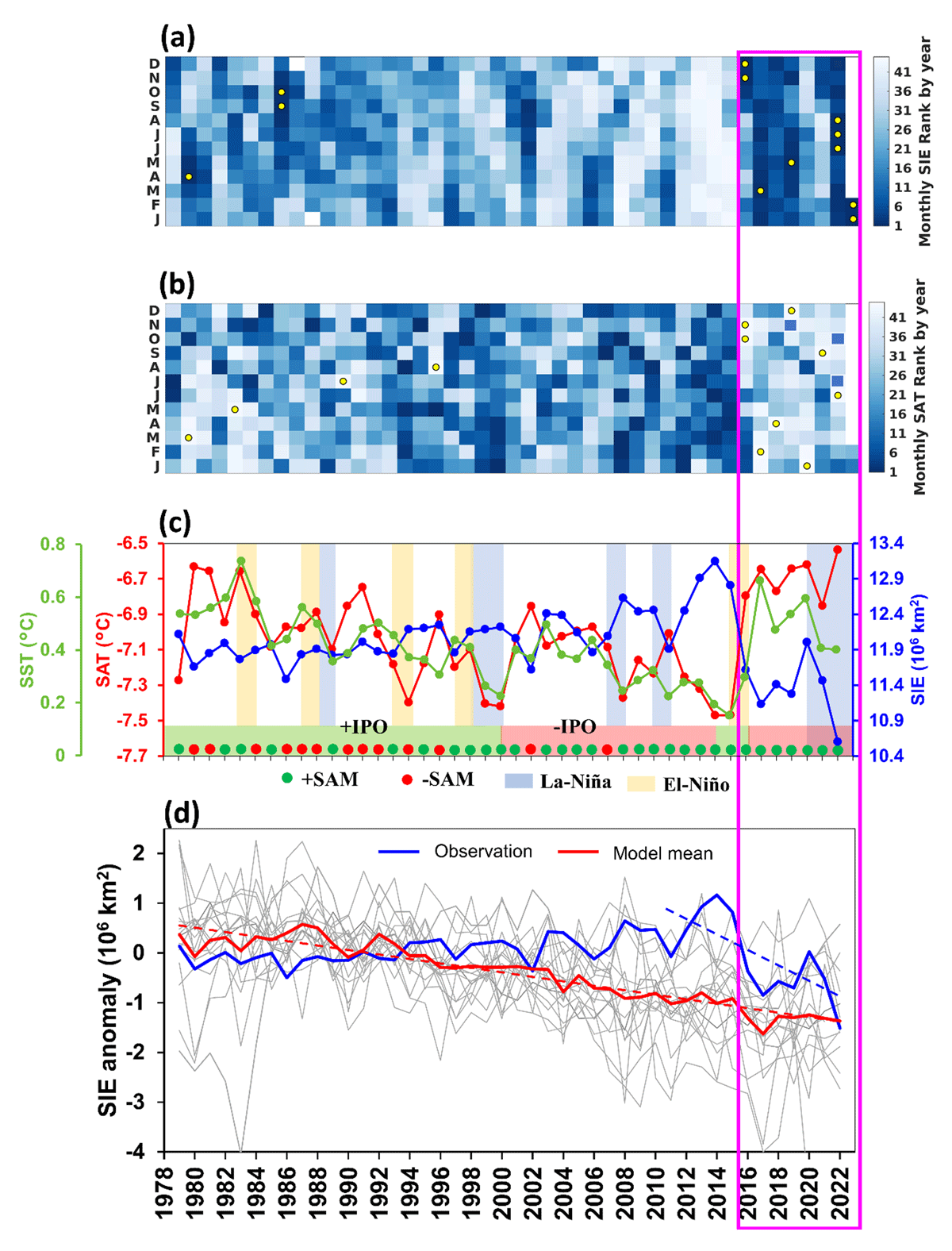
Figure 1
(a) The month-wise ranking of sea ice extents for each year from 1979 to 2023, represented from dark to light shades in increasing order, where a high rank represents high ice extents and lower ranks means lesser sea ice extents. (b) The month-wise ranking of surface air temperature for each year from 1979 to 2023, where a high rank represents higher warming. (c) The annual mean sea ice extents from 1979 to 2022, the corresponding anomalous surface air temperature (SAT), and sea surface temperature (SST) are represented in the blue, red, and green line plots. The green (red) shading represents the dominant positive (negative) IPO phases while green (red) dots represent the annual mean positive (negative) SAM index (Marshall, 2003). The blue (yellow) shading highlights the strong La-Niña (El-Niño) years (d) The yearly sea ice extent anomalies for observational (blue) and the Coupled Model Intercomparison Project Phase 6 (CMIP6) (red) were simulated for the entire Southern Ocean. Anomalies are calculated with respect to the mean from 1979–2015. Observations are based on the merged data from multiple passive microwave satellite sensors available from 1979 to 2022. The dashed blue line indicates the linear trend for observational records from 2010 to 2022 while the dashed red line highlights the long-term trend of sea ice from 1979 to 2022. The CMIP6 sea ice extent anomalies are the r1 ensemble outputs from 20 models (grey) for historical and future simulations with the mean ice extent from multiple models. The yellow-colored points in (a) represent the record low values while it represents extreme high temperatures in (b). The recent decline in sea ice from 2016 to 2023 is highlighted in the magenta-bordered box.
3.1.1 Southern Ocean
Analysis of SIE for the entire Southern Ocean showed a moderate increase in ice extent at an annual average rate of 1.95% decade–1 (significant at 95%) from 1979 to 2015, showing regional and seasonal heterogeneity consisting of increasing and decreasing trends (Figure 1, Table 1). On the contrary, a sudden drop in SIE began in spring of 2016 and the ice extent in the satellite era has reached record lows in 2017, 2022, and now in 2023. Results from the extended time series (1979 to 2022) of SIE showed that the trend has dropped to 0.11% decade–1 and the ice expansion was insignificant (Table 1).
Table 1
Slopes and standard deviations of linear least-squares fit for annual and seasonal sea ice extents in the total Southern Ocean and each of the 5 sectors both for the 43-y record (1979–2022) and in parentheses, for the 37-y record (1979–2015). The values highlighted in bold (bold italic) indicate significance at 99% (95%) or above. The 5 sectors apart of Total Southern Ocean (SO) are, WS: Weddell Sea, IO: Indian Ocean, WP: Western Pacific, RS: Ross Sea, BAS: Amundsen-Bellingshausen Sea.
| SO | WS | IO | WP | RS | BAS | |
|---|---|---|---|---|---|---|
| Annual mean (103 km2/decade) | 14.10 ± 54.65 (235.92 ± 40) | (–0.68 ± 32.17) (80.17 ± 37.18) | 8.47 ± 16.36 (53.20 ± 17.75) | 12.35 ± 11.91 (28.69 ± 15.35) | 34.28 ± 25.44 (110.98 ± 28.40) | (-40.31 ± 15.43) (-37.13 ± 20.26) |
| Annual mean (%/decade) | 0.11 ± 0.45 (1.95 ± 0.33) | (–0.16 ± 0.73) (1.80 ± 0.83) | 0.43 ± 0.83 (2.67 ± 0.89) | 0.99 ± 0.96 (23.02 ± 12.32) | 1.18 ± 0.87 (3.78 ± 0.96) | (–2.72 ± 1.04) (–2.48 ± 1.35) |
| DJF (103 km2/decade) | 7.07 ± 71.73 (250.85 ± 71.37) | 34.22±48.69 (159.66 ± 56.90) | 19.10 ± 18.82 (49.89 ± 23.33) | 15.25 ± 11.47 (29.70 ± 15.25) | 0.90 ± 34.14 (107.48 ± 38.74) | (–62.38 ± 18.08) (–95.87 ± 22.06) |
| DJF (%/decade) | 0.11 ± 1.10 (3.78 ± 1.07) | 1.30 ± 1.85 (5.95 ± 2.12) | 2.52 ± 2.48 (6.48 ± 3.03) | 2.46 ± 1.85 (4.77 ± 2.45) | 0.056 ± 2.14 (6.52 ± 2.35) | (–6.88 ± 1.99) (–10.52 ± 2.42) |
| MAM (103 km2/decade) | 35.75 ± 78.69 (285.69 ± 77.31) | 51.11 ± 45.52 (178.44 ± 53.08) | 25.33 ± 14.67 (52.34 ± 18.56) | 31.94 ± 13.32 (51.21 ± 17.73) | 8.69 ± 37.03 (107.89 ± 42.65) | (–81.34 ± 20.89) (–104.20 ± 23.34) |
| MAM (%/decade) | 0.47 ± 1.05 (3.75 ± 1.01) | 1.88 ± 1.68 (6.47 ± 1.93) | 3.02 ± 1.75 (6.21 ± 2.20) | 3.74 ± 1.56 (6.018 ± 2.08) | 0.39 ± 1.69 (4.83 ± 1.91) | (–8.76 ± 2.25) (–11.02 ± 2.46) |
| JJA (103 km2/decade) | 31.67 ± 55.07 (212.86 ± 48.24) | (–36.80 ± 39.11) (–14.59 ± 49.14) | 2.91 ±26.37 (65.06 ± 31.70) | 16.39 ± 16.76 (24.30 ± 22.70) | 63.21 ± 28.38 (110.59 ± 36.65) | (–14.05 ± 27.05) (27.50 ± 34.32) |
| JJA (%/decade) | 0.19 ± 0.34 (1.31 ± 0.29) | (–0.62 ± 0.66)) (–0.24 ± 0.83) | 0.11 ± 0.96 (2.35 ± 1.14) | 0.96 ± 0.98 (1.43 ± 1.33) | 1.65 ± 0.74 (2.88 ± 0.95) | (–0.70 ± 1.35) (1.36 ± 1.69) |
| SON (103 km2/decade) | 6.59 ± 51.80 (194.72 ± 46.19) | (–4.48 ± 36.48)) (–12.33 ± 46.14) | 4.24 ± 25.84 (59.40 ± 30.20) | (–1.14 ± 22.81)) (8.84 ± 29.54) | 72.23 ± 29.43 (124.35 ± 35.98) | (–5.29 ± 28.49) (14.45 ± 37.22) |
| SON (%/decade) | 0.04 ± 0.29 (1.08 ± 0.26) | (–0.70 ± 0.57)) (–0.19 ± 0.72) | 0.12 ± 0.73 (1.66 ± 0.84) | (–0.63 ± 1.27)) (0.48 ± 1.63) | 1.79 ± 0.73 (3.08 ± 0.89) | (–0.25 ± 1.36) (0.68 ± 1.77) |
The sea ice trend showed a positive slope for all the months (ranging from 25 × 103 km2 decade–1 to 50 × 103 km2 decade–1) except for February (–5.66 × 10³ km2 decade–1), November (–75.47 × 10³ km2 decade–1) and December (–73.66 × 10³ km2 decade–1) from 1979 to 2022 which shows a slightly declining trend (Supporting Figure S1). The exceptional negative sea ice trend in February (1979 to 2022) is mainly attributed to the record low SIE in 2022, which dropped to nearly 31.78% below the long-term average. The monthly rankings of SIE values in the Antarctic showed lower ice extents in the recent years from 2016 onwards, while early years showed higher ice extents (Figure 1a). The top ‘record lowest SIE’ years were observed since 2016, corresponding to the warmest years dating back to 1979. Out of 12 record-low SIE values, 9 monthly lows remained between 2016 to 2022 corresponding to higher warming events after 2015 (Figure 1a–c). It is important to note that the high interannual variability plays an extremely important role in determining the strength and persistence of long-term trends of sea ice (Raphael and Handcock, 2022).
The SIE has declined in all the seasons, with maximum declining trends in summer (7.07 × 10³ km2 decade–1) and spring (6.59 × 10³ km2 decade–1) of 2016–2022 (Table 1). The declining sea ice trends in summer resulted in delayed ice formation in the subsequent autumn and winter seasons (Stammerjohn et al., 2012). Similarly, the decline in SIE in spring leads to extremely low ice conditions in subsequent summer. For example, the sea ice decline observed in spring 2016 and 2021 has led to record low ice conditions respectively for February 2017 and 2022 (John Turner et al. 2020; John Turner et al. 2022)
The SIE during austral spring 2016 recorded a maximum decline at a rate of 75 × 103 km2 day–1 (46% higher than average) from satellite observations (Turner et al., 2017b). The rapid ice retreat during the austral spring 2016 occurred in conjunction with record anomalous atmospheric circulations during the period from September to November 2016. Turner et al., (2017b) noticed that a record strengthening of ASL led to an anomalous decline in sea ice in the Bellingshausen-Amundsen Seas (BAS) and Weddell Sea during September 2016. This was followed by the amplified planetary waves in October 2016 which led to enhanced advection of heat flux to the polar region resulting in an anomalous decline in sea ice in the RS and IO sectors. The largest sea ice decline in November 2016 was due to the record weakening of westerlies (SAM–) that contributed to the higher percentage of sea ice loss in the Weddell and Ross Seas (Meehl et al., 2019; Stuecker et al., 2017; Turner et al., 2017b). Another study suggests that the unusual early breakdown of the stratospheric polar vortex resulted in the record weakening of circumpolar westerlies during Nov-Dec 2016 (Wang et al., 2019). Analysis of the modes of climate variability such as the IPO, suggests that the transition from IPO– (2000 to 2014) to IPO+ (2014 to 2016) along with weakened westerlies and upper ocean warming contributed to the sea ice decline in late 2016 (Meehl et.al. 2019). However, the recent record sea ice decline from 2016 occurred in a dominant IPO– and SAM+, in contrast to the period from 2000 to 2014 which makes it complicated to understand the exact relationship (Figure 1c).
The recent decline in SIE reached record lows in June 2022, July 2022, August 2022, January 2023, and February 2023, which were 13.67%, 9.91%, 6.79%, 39.29% and 39.56% below the long-term average (1979–2015) (Figure 1a). According to John Turner et al. (2022), the previous record low ice extents on 23rd February 2022, highlighted the decline in the Bellingshausen-Amundsen Seas (BAS), RS, and WS. In particular, RS experienced a maximum sea ice decline in response to the deeper ASL favored by La-Niña and positive SAM in October/November 2021. However, very strong El-Niño and negative SAM influenced the anomalously low sea ice conditions over the entire Antarctic with maximum decline in WS in November 2016 (Figure 1c, Turner et al. 2020). The deepening of ASL along with the intense polar cyclones during late 2021 led to greater ice drift from the coastal areas of RS that contributed to the reoccurrence of large coastal polynyas in December and thus record low sea ice conditions in the entire Southern Ocean (John Turner et al. 2022). The recent decline in SIE from 2016 through 2022 contributed dominantly to the overall drop in the trends from 1979 to 2022, considering the satellite observations. It is important to mention here that the physical mechanism of sea ice change in 2016 was different from 2022. Also, the time period and rate of sea ice decline for both years were different for each sector.
Along with the above observational analysis, we have analyzed the SIE simulated by various CMIP6 models. The coupled climate models make an important tool for understanding the sea ice evolution in the past and in future. The CMIP6 outputs are used as a representative tool to complement the recently observed declining trend in sea ice extent. The ensemble-mean SIE showed a consistent decrease from 1979 to 2022. The discrepancy in model and observed sea ice trends could be attributed to high global mean surface temperatures that influence the strong negative trends in CMIP6, possibly due to high climate sensitivity (Roach et al., 2020). Additionally, the internal climate variability that failed to capture the short-term variations in SIE may play a role in the ineffectiveness of CMIP6 models (Polvani and Smith, 2013; Roach et al., 2020; Shu et al., 2020; Zunz et al., 2013). Especially in the Southern Ocean, CMIP models exhibit positive biases in SST (Kostov et al. 2017; John Turner et al. 2013a) and freshwater flux and negative bias in simulating the changes in mixed layer depth (MLD) (Gao et al., 2023; Sallée et al., 2013).
The observed declining trend (–142 × 103 km2 year–1) of SIE in the recent decade (2010–2022) is nearly comparable to the consistent declining pattern of model-based trend (–45 × 103 km2 year–1) (Figure 1). However, the difference in the declining trend between the model and observations could be due to the uncertainty in the record lengths. It has been observed that the sea ice extent in the Antarctic reached closer to the model mean values in 2022 (Figure 1). This suggests that in coming years, the trend in observational SIE might follow the model predictions more closely indicating a possible future shift towards a warmer climate in the Southern Ocean. However, further research and monitoring are necessary to gain a better understanding of the trends in Antarctic sea ice extent considering the uncertainties in climate models.
Even though the SIE for the entire Southern Ocean showed a drastic decline since 2016, there were regional heterogeneities observed in different sectors (Schroeter et al., 2023). The regional and seasonal asymmetries are caused due to the response of different sectors sensitive to ocean-atmospheric forcing for different seasons (S. E. Stammerjohn et al. 2008; S. Stammerjohn et al. 2012; Schroeter et al. 2023). One of the causes for these asymmetries is the delay or early retreat responsible for the growth or loss of sea ice. The timing of sea ice retreat and the following ice advance determines the duration of the summer (ice-free) season; correspondingly, the winter ice season duration varies based on sea ice advance and retreat. The start of early sea ice retreat after the annual maximum on 31st August 2016, fast-paced the rapid ice decline to 2 standard deviations below the mean (Turner et al., 2017b). The poleward advection of heat flux due to the amplified planetary waves led to anomalous sea ice decline in RS and IO regions. In November 2016, the record weakening of westerlies contributed to the largest ice retreat in WS compared to other regions (Turner et al. 2017b). By the end of austral summer, the IO and Pacific sectors have remained nearly ice-free, while WS, BAS, and RS have seen little ice (Turner et al. 2017b).
3.1.2 Weddell Sea
The WS is an exceptional region that contains most of the multiyear sea ice in the Antarctic. The monthly minimum SIE in the WS always occurred in February while the maximum SIE occurred in September for 34 years, in October for 6 years, and in August for 4 years (Supporting Figure S2a). The yearly trend of SIE in the WS experienced a drop from 80.17 × 10³ km2 decade–1 (1979 to 2015) to –0.68 × 10³ km2 decade–1 during the period from 1979 to 2022 with record high SIE in the year 2015 followed by a steep decline (Table 1).
The largest deviation in December 2016 was attributed to the rapid sea ice retreat during 11–15 December 2016, to mark the record negative SIE anomaly (–1.30 × 10⁶ km2) on 15 December (Turner et al., 2020). The emergence of Maud Rise polynya towards the later period of 2016 is one factor contributing to the sea ice decline in the WS. This significant feature reoccurred after 40 years and its initial appearance during the winters of 1974–1976 is discussed earlier (Carsey, 1980).
The pronounced melting of sea ice, however, was sustained through the successive years from 2017–2021, with the maximum in 2017. The anomalous sea ice decline in 2017 is attributed to the opening of a large polynya on the Maud Rise that remained for 79 days (B. Jena et al. 2019; Babula Jena and N. Pillai 2020; Turner et al. 2020). Various studies showed the surface wind stress curl contributed to the enhanced circulation of the subpolar gyres leading to enhanced vertical mixing of salinity and heat from the Circumpolar Deep Water layer (Cheon and Gordon, 2019; Jena et al., 2019; Meehl et al., 2019). This is thought to be an important contributing factor to the weakened stratification and the opening up to the Maud Rise polynya in 2016 and 2017. It was believed that the abrupt increase of sea ice in the year 2020 was the start of sea ice recovery that occurred due to the shorter period of polynya. Analysis of ARGO floats (Float No. 5904468 and 5904472) and model reanalysis data showed that the recent decline in WS sea ice is consistent with surface and mixed layer warming (Figure 3). The float-5904468 located close to Maud Rise, revealed the mixed layer warming to a maximum of 2.5°C during the summer of 2016/2017 (Figure 3a-c). This anomalous oceanic warming is nearly 1.5°C more than temperatures during the summer of 2015–16, which remained consistent in the following years (2018–2020). Also, another float-5904472 showed significant warming (~1°C) at the Maud Rise during 2017 (Figure 3a, 3d and 3e). After 2017, the float drifted westward up to 45° near the multiyear ice, and therefore the mixed layer warming was not visible.
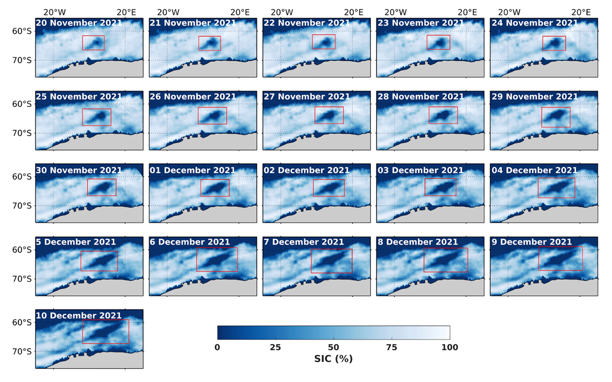
Figure 2
The reoccurrence of Maud Rise polynya (Red rectangle) from 20th November 2021 to 10th December 2021.
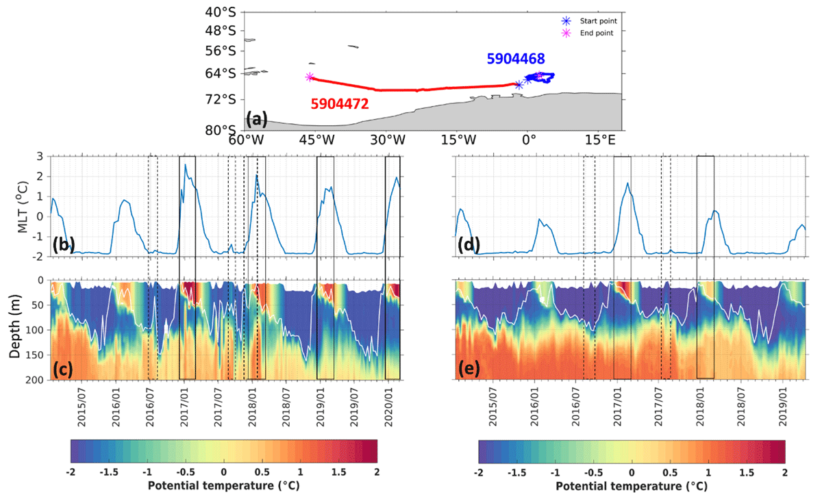
Figure 3
(a) The tracks of selected ARGO floats (id- 5904468 and 5904472) in the Weddell Sea (WS) during the period of consideration, (b) the mixed layer temperature (MLT) and (c) Potential temperature (°C) for float-5904468, (d) the mixed layer temperature (MLT) and (e) Potential temperature (°C) for float-5904472. The white solid line in Figure 3c and Figure 3e shows the variability of ocean mixed layer depth. The black solid boxes indicate the profiles for the austral summer seasons while the black dashed boxes highlight the polynya formation period.
Sea ice in 2021 experienced a sudden decline that deviated greatly from normal with maximum deviation in December (Supporting Figure S2). The ice loss contributed to an increase in the areal extent of open water (Maud Rise polynya) from 4.375 × 10³ km2 (20 November 2021) to 146.875 × 10³ km2 (10 December 2021) (Figure 2). The spread of Maud Rise polynya to east-northeast in 2021 contrasted with the 2016–17 events where the polynya had expanded in a west-southwest direction (B. Jena et. al. 2019). The formation mechanism of 2021 polynya is similar to 2017 (Francis et al., 2020; Jena et al., 2019) with the intrusion of warm and moist air from the tropics by the cyclone with the feature similar to the atmospheric river (AR). On 17th November, an extratropical storm was formed in the north-western part of the Weddell Sea with a center of low pressure at approximately 40°S and 46°W (Supporting Figure S3). This cyclone transported anomalously large moisture and heat from midlatitudes along a meridional track impacting sea ice over the Weddell Sea on the 19th and 20th of November, creating a favorable condition for polynya formation (Francis et al. 2020; Jena et al. 2022a). From 16 to 20 November 2021, the IWVF along the cyclonic track observed anomalous transport of moisture-laden air masses with values exceeding 300 kgm–1s–1 on 19th November 2021 (Supporting Figure S3a-e). This AR event was marked by anomalous atmospheric warming with a daily record increase in SAT (black dashed contours) from 16 to 20 November (Supporting Figure S3f-j). The strong moisture-laden warmer northerly winds associated with AR increased the SAT (>0.2°C) and contributed to the anomalously low SIE (due to the melting of sea ice), promoting the opening of MR polynya (Supporting Figure S3k-o). Simultaneously, the oceanic conditions contributed to the formation of MR polynya. The presence of MR seamount that limits the water depth in this region and the entrainment of warm water to the surface through Weddell gyre provided ideal conditions for the sea ice to be thinner and lower even during winter (Jena et al., 2019).
The open ocean polynyas act as a window through the pack of sea ice, allowing a massive gain of net heat flux by the ocean that occurred during the spring and summer of 2016, 2017, and 2021 (Supporting Figure S4). Furthermore, when heat loss to the atmosphere increases, these polynyas are also characterized by large amounts of sea ice production due to the restratification of fresh water to the surface (Dufour et al., 2017; Ohshima et al., 2013). The Maud Rise polynya in 2017 produced ~200 km3 of new sea ice (Zhou et al., 2023).
3.1.3 Indian Ocean
The Indian Ocean showed the maximum monthly SIE mostly in the month of October followed by September (Supporting Figure S5a). In most years, the monthly minimum SIE was observed in February while it occurred in March for six years (Supporting Figure S5a). After observing the third-highest SIE (4.22 × 10⁶ km2) in October 2014, it experienced a dropdown in SIE to a record-low value in February 2016 (0.12 × 10⁶ km2) (Supporting Figure S5a). The annual average trend in SIE dropped from 53.20 × 10³ km2 decade–1 (1979 to 2015) to 8.47 × 10³ km2 decade–1 (1979 to 2022) which deviated to the lowest in November 2016 (Table 1 & Supporting Figure S5a). Compared to the trend from 1979 to 2015, the lowest trend was observed in winter (2.91 × 10³ km2 decade–1) followed by the trend in spring (4.24 × 10³ km2 decade–1) during the period from 1979 to 2022 (Table 1).
3.1.4 Western Pacific
In the Western Pacific, monthly maximum SIE is observed in September for 18 years, October for 15 years, and August for 10 years, wherein the minimum sea ice is observed in February most of the time, except for 4 years (1980, 1985, 1986, 2017) when it occurred in March (Supporting Figure S6a). The largest monthly deviation (~ –0.71) was observed in the month of September-October 1989, while the sea ice in September-October 1982 showed the largest positive deviation (Supporting Figure S6a). The annual average SIE showed an increasing trend till 2015 (28.69 x 10³ km2 decade–1) to set a record high value in 2013 (1.52 x 10⁶ km2). The SIE drop after 2015 contributed to the decline in the annual ice extent trend to 12.35 x 10³ km2 decade–1 from 1979 to 2022. The annual average SIE marked the second lowest in 2022 following the record low value in 2002 (Supporting Figure S6a).
3.1.5 Ross Sea
Sea ice in the Ross Sea sector experienced a large monthly variability, with the maximum in October for 14 years, September for 19 years, August for 8 years, and July for 3 years (Supporting Figure S7a). Considering the 43-year record, the sea ice trend showed the maximum decline to 34.28 x 10³ km2 decade–1 (1979–2022) from 110.98 x 10³ km2 decade–1 (1979–2015) corresponding to the decreases in the summer and autumn seasons. During the retreat season, the sea ice trended down to 0.90 x 10³ km2 decade–1 (1979–2022) from 107.48 × 10³ km2 decade–1 (1979–2015) (Table 1). The RS reached a record-low SIE (0.07 × 10⁶ km2) in February 2017, where a higher positive standard deviation was noted in January 2015 and remarkably lower values in March 2017 and March 2022 (Supporting Figure S7a). Both the RS and BAS experienced a nearly ice-free state during February and March 2022 (Figure 4). The occurrence of large polynya in the RS in 2021 was one of the factors responsible for the recent decline of sea ice through ice-albedo feedback (John Turner et al. 2022). The areal extent expanded from 1250 km2 on 26th November 2021 to 15000 km2 on 5th December 2021 (Supporting Figure S8). Also, the period after 2015 showed strong negative wind stress curl in winter, which created favorable conditions for upwelling and mixing of sub-surface warm water into the surface (Supporting Figure S12). Overall, the RS SIE decline from 2016 to 2022 was consistent with the upper ocean warming observed from model reanalysis data (Figure 8).
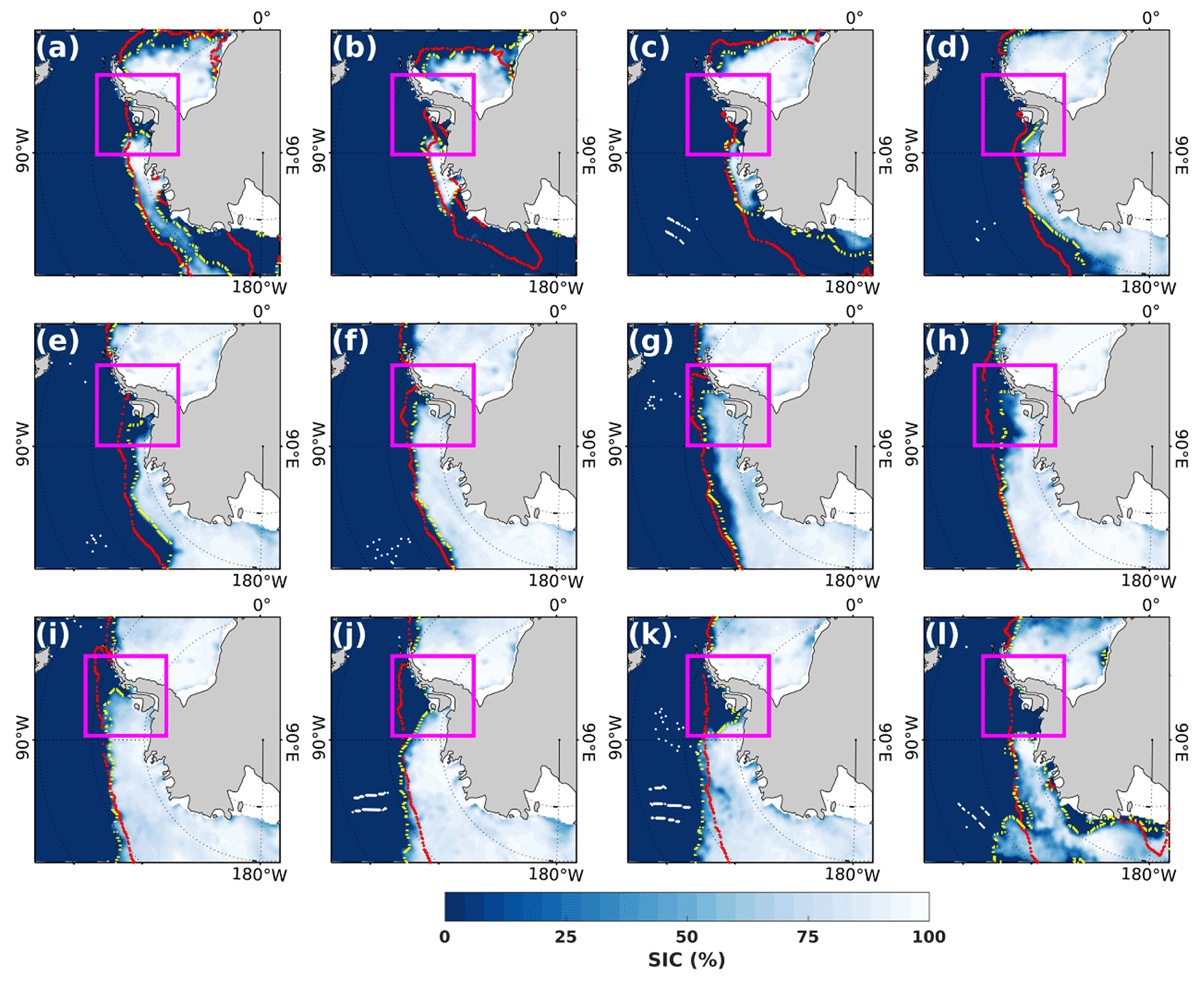
Figure 4
(a-l) Sea ice concentration (SIC) for the 15th day of each month sequentially from January to December 2022 in the western Antarctic region. The yellow line represents the sea ice edge for the 15th day of each month from January to December 2022. The red line indicates the daily climatological sea ice edge (median) from 1979 to 2015. The magenta square highlights the region of western part of Antarctic Peninsula that remained nearly ice-free throughout 2022 with the sea ice concentrations below the long-term median values.
3.1.6 Bellingshausen-Amundsen Sea
The Bellingshausen-Amundsen (BAS) has a climatological low-pressure region that lies between the Antarctic Peninsula and the RS, induced by the unique orography of the Antarctic (Hosking et al., 2013). The maximum monthly SIE was observed in September for 21 years, in August for 17 years, in October for 3 years, and in July for 3 years (Supporting Figure S7c). The recent years (2016, 2018, 2019, 2021) experienced the maximum SIE in August, while generally, it occurred in September. The annual average SIE showed a declining trend of –40.31 x 10³ km2 decade–1 (1979 to 2022), as compared to –37.13 x 10³ km2 decade–1 (1979 to 2015) with a maximum declining trend in winter and spring seasons (Table 1). The declining trend of SIE before 2010 was observed with a record low value in 2007, followed by an upward trend after 2010 (Supporting Figure S7c). Notably, the winter season of 2022 has recorded the lowest sea ice extent (1.53 × 10⁶ km2) over the entire satellite period, which highlights the declining trend of SIE in this region (Supporting Figure 7d). Additionally, the spring season observed the second-lowest SIE in 2022 after the record lowest in 2017 (Supporting Figure 7d). The monthly deviations illustrated the higher positive values in September 2015 and the lowest in May 2017, June 2017, and August 2022 (Supporting Figure S7c).
In 2022, the western part of the Antarctic Peninsula experienced a drastic decline in sea ice and remained ice-free all year long (Figure 4). Such kind of anomalous features occurred due to the increased air temperature and locally enhanced winds along with the northerly warm winds, causing the sea ice to retreat in the Ice shelf front (Massom et al., 2018). The reduced sea ice in the region of ice shelf fronts leads to extensive open-ocean conditions to large-scale disintegration of ice shelves along the western Antarctica Peninsula through basal melting by ocean heat flux and mechanical breaking from large Southern Ocean waves (Massom et al., 2018; Wille et al., 2022).
3.2 Sea ice variability from 2016 to 2022
The analysis of SIC maps showed an overall negative ice anomaly from 2016 to 2022, with a regional heterogeneity consisting of both negative and positive anomalies (Figure 5). The negative SIC anomaly in summer is marked as highest in the WS, the eastern part of RS that continues to some extent in the western part of BAS, and also in the coastal parts of the IO sector (Figure 5a). During summer, the pronounced negative ice anomaly in the WS is caused by the presence of anomalously low pressure over the Antarctic and high pressure in the north, which played a role in advecting warm and moist air from the midlatitudes (Figure 5a; Turner et al. 2020; John Turner et al. 2022). The cyclonic pattern depicting the low MSLP region observed in the Weddell Sea promoted ice transport around the Weddell Gyre and to the east of Antarctic Peninsula (Turner et al., 2020). The strengthening of Weddell Gyre due to intense westerly winds promoted the increased advection of sea ice to the southwest of Weddell Sea. The sea ice then moved northward along the eastern part of Antarctic peninsula. The record westerly winds near Antarctic Peninsula in September 2016 caused anomalous advection of sea ice from the north-western Weddell Sea leading to extensive reduction of sea ice in this region. Subsequently, in November 2016, a record negative SAM index resulted in unusual warm north-easterly winds into the Weddell Sea that helped to further sustain the negative ice anomalies (Turner et al. 2020). In autumn, there was pronounced sea ice loss along the Southern Ocean except in some parts of IO, WP, and RS whereas the winter season experienced extensive ice loss in WS, BAS, and IO regions (Figure 5b, Figure 5c). The anomalously low sea ice in autumn and winter is attributed to the strengthening of ASL which is a part of Zonal Wave 3 (Turner et al., 2017a). The negative sea ice anomalies are prominent in all the seasons except for the northern part of the Ross Sea in winter and spring (Figure 5). During the spring season, sea ice concentration (SIC) anomalies in the eastern part of the Bellingshausen Sea were below average, while the northern part of the Amundsen-Ross Sea sector showed above-average sea ice concentrations (Figure 5d). This dipole sea ice condition was influenced by the strong cyclonic activity in BAS (specifically during 2022) which promoted the anomalous northward flow of cold winds from the Antarctic over the Amundsen-Ross Sea sector while the warm northerly winds blowing to the eastern part of BAS (Figure 5d).
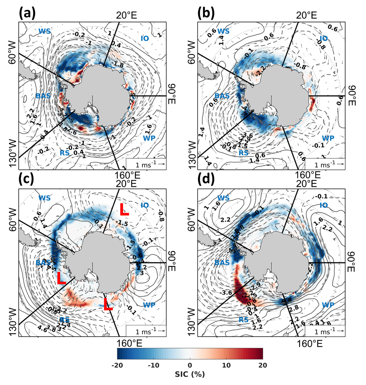
Figure 5
The seasonal average anomaly of sea ice concentration (SIC) (%) composite from 2016 to 2022 overlaid by the anomalies of mean sea level pressure (MSLP) contours and wind directions (grey arrows) for (a) summer (DJF), (b) autumn (MAM), (c) winter (JJA), and (d) spring (SON). The atmospheric pressure lows are indicated with the ‘L’ symbol in red. The dashed line contours represent the negative MSLP anomaly and the solid line contours represent the positive MSLP anomaly. The anomaly is computed with respect to the climatology from 1979 to 2015.
The sea ice variability in the winter and spring seasons follows a nearly heterogeneous pattern of higher and lower concentrations, while a distinctive feature of three atmospheric lows and highs is detected in the winter season (Figure 5c). These are the Rossby waves (planetary waves) with zonal wave number 3 pattern, which is significant during the periods of ice growth and expansion. The ZW3 pattern is marked by three alternating low (troughs) and high (crests) atmospheric pressure with centers located in the Indian, Pacific, and Atlantic sectors that influence the temperature difference between the atmosphere and the ocean (Figure 6c, Raphael 2004; van Loon and Jenne 1972). The net sensible heat flux (SHF) that describes the energy transfer between the atmosphere and the ocean is affected by the temperature difference. The positive (negative) SHF observed in the regions of colder air (warmer air) is associated with increased (reduced) ocean heat loss and more (less) sea ice (Raphael, 2004). The variability in temperature gradient determines the amplitude of ZW3, where the large gradient shows the enhanced zonal wave 3 patterns. The next section describes in detail the role of atmospheric planetary waves on the observed sea ice decline.
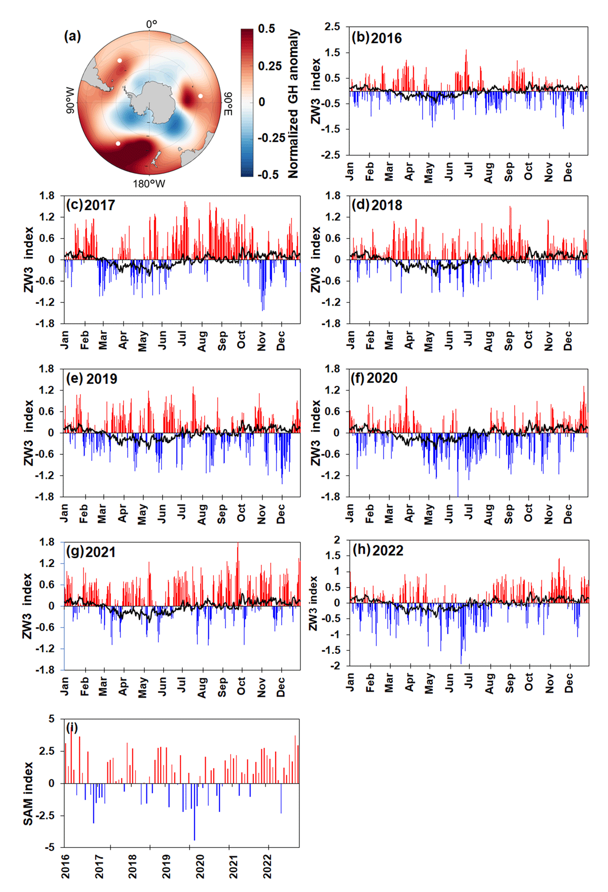
Figure 6
(a) Normalized anomaly of 500 hPa geopotential height (GH) composite from 2016 to 2022 relative to the climatology from 1979 to 2015. White dots represent the locations used for computing the ZW3 index. ZW3 index computed using daily geopotential height at 500 hPa for (b) 2016, (c) 2017, (d) 2018, (e) 2019, (f) 2020, (g) 2021, (h) 2022 based on the methodology by Raphael (2004). The black line represents the ZW3 index computed for the climatological mean from 1979 to 2015. The three ridge points for the analysis are 79.5°E, 32.25°W, and 139.5°W at 45°S latitude (Francis et al., 2019). (i) Monthly SAM index from 2016 to 2022.
3.3 Impact of atmosphere and ocean on the observed sea ice decline
Atmospheric zonal wave is one of the important features affecting the extratropical atmospheric circulation that impacts strongly on the poleward distribution of heat and moisture, Antarctic sea ice, and the atmospheric blocking events (Raphael, 2007, 2004). To understand the response of atmospheric dynamics on sea ice, a detailed investigation was carried out by computing the daily variability of ZW3 index from 2016 to 2021 in the Southern Ocean. The variability of the ZW3 index showed significantly higher values after 2015 greater than the climatological mean, indicating the dominant meridional flow, whereas the negative index represents the more zonal flow (M. N. Raphael 2004, Figure 6). This unusually higher positive ZW3 during 2016 marked a sea ice decline in the BAS, WS, western IO, and WP sectors of the Southern Ocean (Schlosser et al. 2018; Turner et al. 2017b). The record low SIC from September to December 2016 is attributed to the sequential occurrence of events. It includes the weakening of the polar vortex due to planetary waves in early spring that enhanced low SAM conditions and weak westerlies (Schlosser et al., 2018; Wang et al., 2019). Subsequently, the occurrence of negative IOD conditions during Sept-Oct and a strong MJO during November 2016 progressed the decline (Meehl et al., 2019; Wang et al., 2019). Of the overall period, 2017 marked an unprecedented sea ice decline. The amplification of ZW3 patterns (Figure 6b) and negative SAM index corresponds to the anomalous sea ice decline during January–February–March of 2017. The ice-free regions in WS due to the increased absorption of shortwave radiation caused by the westward expansion of MR polynya in late 2016, influenced the anomalous sea ice decline in WS to a record lowest SIE in the summer of 2017 (Supporting Figure 4). The negative MSLP between RS and Amundsen contributed to the lowest SIE in March 2017. The occurrence of intensified extra-tropical cyclones in winter is attributed to the poleward intrusion of warm air associated with the deepening of atmospheric troughs and blocking highs of ZW3 with an increased temperature gradient (Francis et al., 2019). These high-intensity cyclones along with the AR observed anomalous transport of moisture-laden air masses, that drifted sea ice away from the ice pack, causing the Maud Rise polynya to recur in the WS during September 2017 (Campbell et al., 2019; Francis et al., 2019). For example, the amplification of the ZW3 pattern during March–April 2018 due to the asymmetric distribution of pressure patterns increased the meridional influx of heat towards the south, possibly accelerating the sea ice decline over the WS and the RS (Figure 6c). An increase in zonal wave activity hampered the rate of freezing in winter with negative ice anomalies in the IO, WS, and WP. The drop in overall MSLP during November and December 2018 contributed to the record-high air temperature over the Southern Ocean (Turner et al., 2020).
The sea ice reduction in autumn 2019 is attributed to the occurrence of a series of polar cyclones during April-May 2019, and its impact on the upper ocean through dynamic and thermodynamic processes (Jena et al. 2022a, Jena et al. 2022b). The warming of the ocean mixed layer in autumn 2019 occurred due to the net gain of heat flux by the ocean. The ZW3 index was in its positive phase for most of the days from March to May 2019 (Jena et al. 2022a). This led to the amplification of large zonal temperature gradients which in turn created the conditions of baroclinic instability. This instability played a role in the formation of explosive polar cyclones during April/May 2019, which influenced the sea ice condition (Jena et al. 2022a; Francis et al. 2019; Francis et al. 2020). While the wave amplification in the polar middle atmosphere usually happens during winter, it occurred at lower altitudes in 2019 than in previous years (Yamazaki et al., 2020). The stratospheric warming due to disrupted weather systems during winter weakened the polar vortex permitting the intrusion of warm air, thereby reducing the depletion of ozone in spring (Gray and Stein, 2019). The increased stratospheric temperatures along with the occurrence of explosive polar cyclones advected the warm air from the mid-latitudes into the ice-covered region, resulting in anomalous sea ice decline during spring (Gray and Stein, 2019).
The annual mean SIE in 2021 observed a noticeable drop of 0.65 million km2 below the mean (1979 to 2015). The SIE decline had a remarkable effect on the WS, RS, and IO which reached the lowest ice extent in late 2021. The sea ice decline during spring 2021 observed the dominant contribution of intensified zonal wave 3 (Figure 6g). The anomalous convection in the southwestern subtropical Pacific due to the presence of La-Niña, triggered the poleward propagation of the Rossby wave train from eastern Australia (Zhang and Li, 2023). The presence of atmospheric rivers during 16-20 November 2021 also contributed significantly to sea ice lows during spring 2021 (Supporting Figure 3, Refer to section 3.1.2). ZW3 index and sea ice cover during spring 2021 showed a significant negative correlation (p < 0.05) through the changes in surface air temperature and water vapor (Supplementary Figure S10). The amplified atmospheric waves, along with the SAM+ index, generate higher temperature gradients leading to the formation of intense storms promoting the poleward transport of heat (Pezza et al., 2012). The atmospheric warming during winter/spring 2021 persisted in 2022 as well (Turner et al., 2022; Zhang and Li, 2023). The Antarctic as a whole experienced a record low SIE in 2022, attributed to the negative sea ice anomalies in all the seasons except for RS (Figure 1). The low sea ice cover during autumn is attributed to the strengthening of low pressure in the Amundsen Sea which is a part of ZW3. The higher ZW3 amplification associated with positive SAM and strong La-Niña conditions during spring influenced the dipole sea ice behavior in the northern part of Amundsen-Ross Sea and the eastern part of Bellingshausen Sea (Figure 6, Figure 5).
We have quantified the impact of atmospheric zonal wave intensification on the reduction of sea ice cover since 2016. Our analysis focused on examining the co-variability between the ZW3 index and the different climatic variables that contributed to the sea ice variability. The intensification of ZW3 generally starts from autumn to the maximum in winter followed by the secondary maximum index during spring seasons (Raphael 2004; Turner et al. 2017a). The pattern of correlation of the ZW3 index with total column water vapor (Supporting Figure 9a) during winter (JJA) and spring (SON) of 2016 to 2022 showed a clear wave 3 patterns indicating that in poleward flow regions, the SAT is warmer and hence increased sea ice melting during positive phases of ZW3 with 95% significance (Supporting Figure 9b, Supporting Figure 9c). The strong poleward flow of warm air, induced by ZW3, can cause warmer upper layers of the ocean and a deeper mixed layer, potentially inhibiting the formation of sea ice (Supporting Figure 9d, Raphael, 2007). Also, the intensification of zonal waves correlates significantly (p < 0.05) with the atmospheric warming in summer (DJF) of 2016-2022, which reflects the sea ice decline over the entire Southern Ocean (Supporting Figure 9b, Supporting Figure 9c). The atmospheric warming observed during austral summer (DJF) might be due to intrusions of midlatitude air associated with wave number 3 intensification in preceding seasons (Supporting Figure 9b, J. Turner et al. 2002; J. Turner et al. 2003). It has been noted that the positive phase of SAM during summer reduced MSLP in the BAS region where one of the wave number 3 troughs is climatologically located, has contributed to an increase in the amplitude of wave number 3 (Fogt and Zbacnik, 2014; Turner et al., 2017a). Recently, the intensifying SAM, which includes a zonal wave-3 structure within it, has shifted toward its asymmetric component (Campitelli et al., 2022; Schroeter et al., 2023; van Loon and Jenne, 1972; Wachter et al., 2020). As a result, there has been an increase in poleward meridional flow over the sea ice zone. During fall/autumn (MAM), we observe a significant positive correlation (p < 0.05) of the ZW3 index with the total column water vapor (Supporting Figure 9a). The intensified anomalous poleward flow of warm air that indicated a clear signal of the ZW3 pattern is one of the factors that might have influenced the circumpolar decline in sea ice significantly (Supporting Figure 9c).
The poleward propagation of Rossby waves enables the teleconnection between ENSO and the extra-tropical climate (Turner et al., 2017b). In general, these waves are well developed during winters of the Southern hemisphere with higher geopotential heights during the El-Niño phase (Karoly, 1989; Kiladis, 1998). This wave train affects the western part of the Antarctic, an area close to ASL, coincident with one of the climatological ridges of wave number 3 troughs (Turner et al., 2017a). ENSO plays a significant role in determining the depth of the ASL. ASL is a region where the strongest tropical-Antarctic teleconnections exist, and these tropical effects have a significant influence on the Rossby waves (Li et al., 2021; Turner et al., 2017a). As the latitude of the ASL reflects the meridional location of the southern hemisphere storm track associated with large-scale modes such as SAM, it is likely to play a substantial role in surface winds around Antarctica (Turner et al., 2013b). The longer time effect of ENSO showed intense warming over the tropical Atlantic, which results in the generation of Rossby waves and thus deepening of ASL, similar to the effect generated by the tropical Pacific Ocean (Turner et al., 2017a). Recently, the low sea ice conditions from 2019 to 2022 occurred in the La-Niña state of ENSO. A combination of the positive phase of SAM and La-Niña conditions favors deeper ASL, resulting in anomalously strong southerly winds to more equatorward sea ice transport (Fogt et al., 2012; Li et al., 2021). Strong upper ocean warming in the western Pacific during the winter of 2021 promoted the formation of La Niña, which led to the anomalous rise in SST in the southwestern subtropical Pacific (Zhang and Li, 2023). This warming triggered deep convection in the southwestern subtropical Pacific, which resulted in the formation of the Rossby wave train originating from eastern Australia and propagating south-eastwards, ultimately leading to the deepening of the Amundsen Sea Low (Zhang and Li, 2023). As a result, Antarctic Peninsula and the West Antarctic experienced warmer air advection. The deeper ASL along with the intense polar cyclones led to greater ice drift from coastal areas of the Ross Sea that contributed to the reoccurrence of large coastal polynyas and thus record low sea ice conditions during spring 2021 (John Turner et al. 2022). Additionally, in December 2021, the low MSLP in the Weddell Sea and high pressure in South Atlantic caused stronger west to north-westerly winds across the Weddell Sea, leading to increased ice export (Turner et al., 2022).
3.3.1 Influence of anomalous water vapor and air temperature
The seasonal total column water vapor anomalies for the period from 2016 to 2022 are shown in Figure 7. The higher amount of vapor content over the Southern Ocean represents an increased poleward transport of warm air elevating the air temperature in this region. The occurrence of troughs over the Southern Ocean influences the northerly transport of moisture. The seasonal circulation, vapor transport, and SAT anomalies represent the southward flow of warm air that results in warming across all seasons. The higher air temperature (~0.5°C) observed in summer corresponds to reduced sea ice cover in the WS, RS, IO, and to some extent in the BAS region (Figure 7e). The SAT (>1°C) in the autumn season associated with the low MSLP anomalies experienced anomalous warming in the RS, WS, BAS, and IO regions (Figure 7f). Similarly, the winter season was marked by pronounced warming in the IO sector, BAS, western WS, and RS, while cooling in the WS and WP. The northerly transport of warm winds associated with a significant decline in MSLP enhanced the sea ice decline in the IO sector during winters (Figure 7g). The anomalous low MSLP over the whole Southern Ocean during spring boosted the sea ice decline mostly in WS, IO, and RS (Figures 7h and Figure 5).
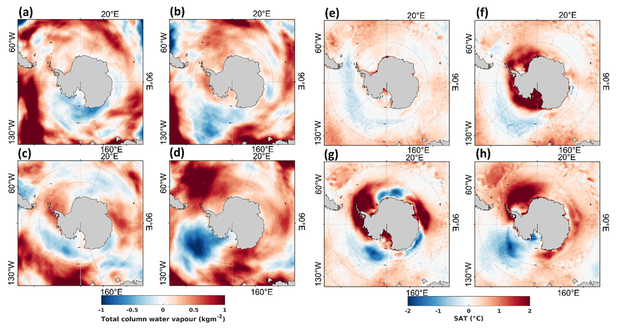
Figure 7
The seasonal average anomaly of total column water vapor (a-b-c-d) and, surface air temperature (e-f-g-h) composite from 2016 to 2022 for (a and e) Summer (DJF), (b and f) Autumn (MAM), (c and g) Winter (JJA), and (d and h) Spring (SON) seasons. The anomaly is computed with respect to the climatology from 1979 to 2015.
3.3.2 Influence of ocean warming
The coupling between the ocean and atmosphere processes occurs through the exchange of heat, moisture, and momentum. Figure 8 shows the seasonal SST and MLT anomalies for the period from 2016 to 2022. Observing the Southern Ocean as a whole, the SST deviated largely from the mean values during summer with the maximum positive anomaly of ~0.6°C in WS and IO corresponding to the declining pattern of the SIC (Supporting Figure S13). The MLT warming in summer recorded an increase of more than 0.5°C dominantly in the WS, RS, and IO regions (Figure 8e). Low sea ice cover in summer is associated with the anomalous gain of shortwave radiation flux and net heat flux into the ocean during spring and summer (2016–2022) (Supporting Figure S11). During this period, anomalous increase (>0.5°C) in ocean-atmospheric temperatures is more widespread rather than being concentrated solely in the polynya region. However, the gain of heat flux and warming is more intense in the polynya regions such as WS and RS (Figures 2, 5a, 8, Supporting Figure S4, Supporting Figure S11). In parallel, negative wind stress curl favored anomalous warming of the mixed layer by the upwelling of subsurface warm water during winter in the RS and BAS (Supporting Figure S12) hindering thermodynamic growth of sea ice and leading to reduced summer SIE (Figure 5a). The surface oceanic warming in the summer further leads to a delayed sea ice formation in the following growth season reducing the overall sea ice cover (Jena et al. 2022a).
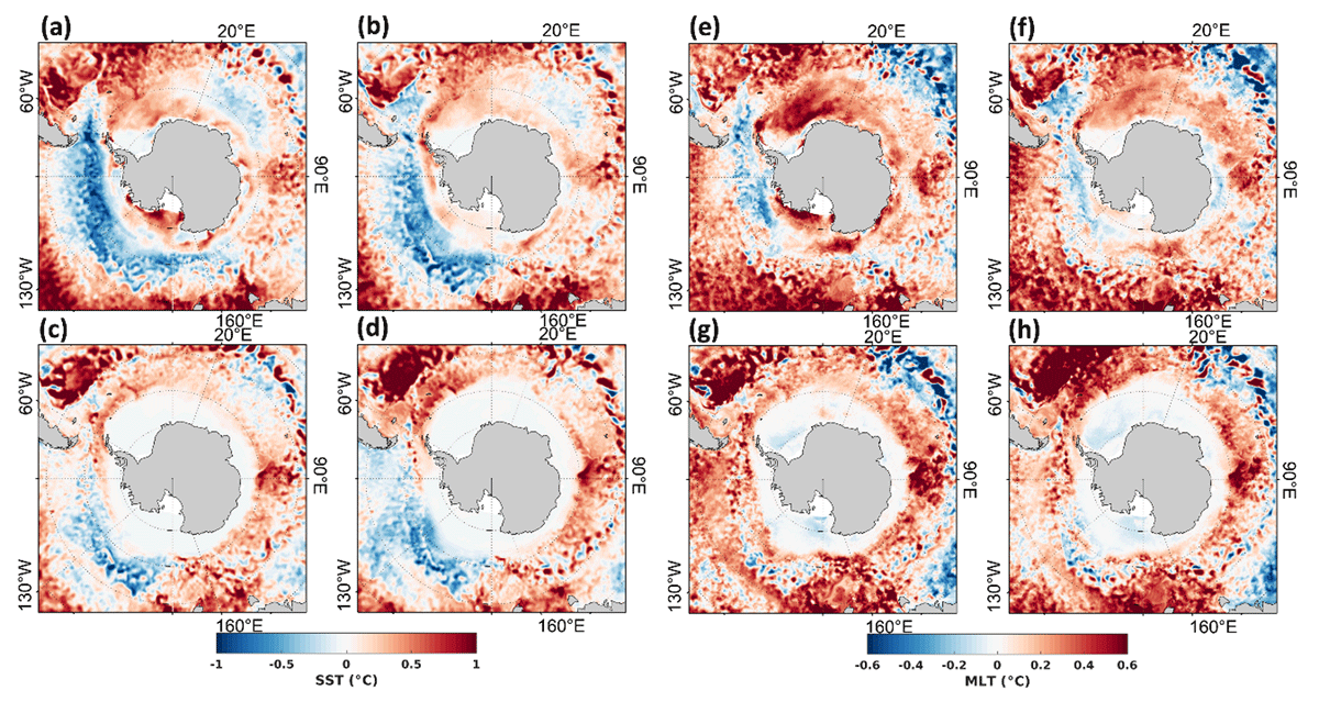
Figure 8
The seasonal average anomaly of sea surface temperature (a-b-c-d) and, mixed layer temperature (e-f-g-h) composite from 2016 to 2022 for (a and e) Summer (DJF), (b and f) Autumn (MAM), (c and g) Winter (JJA), and (d and h) Spring (SON) seasons. The anomaly is computed with respect to the climatology from 1979 to 2015.
The observed SST and MLT variability during 2016-2022, was likely resulted from the integrated influence of regional and remote ocean-atmospheric processes. The upper ocean temperatures in the Southern Ocean can be modulated by the strengthening and shifting of winds. The westerly winds that are responsible for driving the circulation pattern around Antarctica are associated with the SAM perturbations.
4. Conclusion
The rate of SIE increase in the Southern Ocean from 1979-2022 has declined more than five times as compared to the decadal expansion during 1979–2015, with the rapid decline starting since 2016. This decline in annual average ice expansion from 2016 to 2022 recorded a drop of around 2.6 million km2 below the long-term mean during 1979–2015. The lowest sea ice cover was however seen during 2016-2022, with a reduction of the ice extent to the record lowest value (10.60 × 10⁶ km2) in 2022 followed by the second lowest (11.12 × 10⁶ km2) in 2017. An increase in sea ice during 2020 was assumed to be the start of recovery however, there was a sudden drop in 2021 and 2022 (summer, autumn, and winter), similar to the situation in 2017. In response to the pronounced decline, the SIE reduced predominantly in the WS and RS, with the occurrences of rare polynyas from 2016 to 2021. The decrease in SIE specifically in WS is linked to the ocean-atmospheric warming as detected by both Argo floats and model reanalysis data. The sea ice on the western part of the Antarctic Peninsula declined dramatically and remained ice-free in 2022. We find that the unusual variability in SIE occurred due to the combined influence of the intensification of the atmospheric zonal waves, anomalous increase in air temperature, water vapor, and warming in the ocean mixed layer. However, it is important to mention here that the physical mechanism of record low sea ice conditions in 2022 was different from 2016/17. During 2022, the Ross Sea contributed maximum to the record low sea ice anomalies in Antarctica, due to the strengthening of ASL favored by La-Niña and positive SAM in October/November 2021. In contrast, anomalously low sea ice conditions prevailed over the entire Antarctica in a very strong El-Niño period and negative SAM during November 2016. The response of tropical forcing to sea ice changes may not occur similarly as each El-Niño and La-Niña event is unique in terms of their spatial structure and seasonal evolution; therefore, their impact on sea ice might not be the same. Hence, future studies are required to understand the contrasting influence of ENSO events on Antarctic sea ice.
CMIP6 models showed a consistent declining trend in SIE, similar to the trends from satellite observations since 2016, which could hint at a possible shift towards a warmer climate regime. Although it is difficult to provide a conclusive statement on whether the observed trend is the start of SIE decline as predicted by the CMIP6 models, the findings from this article confirm the repeated anomalous SIE decline started from austral spring 2016 and continued till 2022 and early 2023, with a background of anomalous ocean-atmospheric warming. Considering the current climate changes in and around Antarctica, the variability of regional ocean-atmospheric circulation and sea ice cover influenced by major climate oscillators like IPO and SAM are important. Even though the sudden SIE decline in late 2016 was attributed to the transitional shift from IPO– (2000–2014, increase in sea ice) to IPO+ (2014–2016), the cause of record low SIE during 2016–2022 in a setting of dominant IPO– and SAM+, needs future investigations to determine how the climate change will affect the Antarctic sea ice.
Data Accessibility Statements
All data analyzed in this study are publicly available and the links are provided in the ‘Materials and Methods’ section.
All the codes used in this study are available on request from the corresponding author.
Additional File
The additional file for this article can be found as follows:
Ethics and Consent
This article does not contain any studies with human or animal participants performed by any of the authors.
Informed consent was obtained from all individual participants included in the study.
Acknowledgements
We gratefully acknowledge the Director, National Centre for Polar and Ocean Research (NCPOR), Goa, for their motivation and encouragement to carry out the research. We sincerely acknowledge various organizations such as National Snow and Ice Data Center (NSIDC), National Oceanic and Atmospheric Administration (NOAA), European Centre for Medium Range Weather Forecast (ECMWF), National Centre for Atmospheric Research (NCAR), and Asia-Pacific Data-Research Center (APDRC) for making various datasets available in their portals. Kshitija S., a Ph.D. student acknowledges the financial support from the MoES Research Fellow Program for carrying out this study. This research is supported by the NCPOR and the Ministry of Earth Sciences. We are sincerely thankful to the editor and the anonymous reviewers for conducting a rigorous peer-review process that helped to improve the quality of the paper. This is NCPOR contribution number J-11/2023-24.
Funding Information
Kshitija S. acknowledges the financial support from the MoES Research Fellow Program for carrying out this study. This research is supported by the NCPOR and the Ministry of Earth Sciences.
Competing Interests
The authors have no competing interests to declare.
Author Contributions
Kshitija S: Conceptualization, designed the analysis, and wrote the manuscript. B. Jena: Supervision and data interpretation. All four authors revised the manuscript and interpreted the results.