
1. Introduction
Downstream development of linear and non-linear instability has a long history in hydrodynamics. In the real atmosphere, the great development of the general large-scale movement is often linked to the baroclinic nature of the atmosphere. Consequently, there is a need to discuss conditions of baroclinic shear current instability (Stewartson and Stuart, 1971; Hocking et al., 1972). In order to make the results of the research more generally, the context of the research is more consistent with the present situation. In our stream function, U is a function of latitude y, and the effects of zonal shear flow and beta on baroclinic instability are considered, where the curvature of zonal flow can modify the background potential vortex gradient (effective β). In the Pedlosky article (2019), by selecting the stream function, U in the stream function selects a constant, which is represented as the mean value of atmospheric motion. The choice of shear flow is only one particular case and does not have any generality.
Charney (1947) and Eady (1949) formulated a model of baroclinic instability, they indicated that the disturbance viewed in the atmosphere and ocean could be interpreted as a manifestation of baroclinic instability of the basic zonal flows. A simple two-layer model with a small vertical scale to remove interference was introduced by Phillips (1954). Lin (1955) and Drain et al (2004) studied the stability of unidirectional flows when β is zero. Drazin et al. (1982) have shown Rossby waves modified by the basic shear in a barotropic model. In recent decades, many meteorologists (Pedlosky, 1976; Pedlosky and Polvani, 1987; Polvani and Pedlosky, 1988) have done plenty of discussions on it and obtained a broad research topic. In new research, topographic slopes and the quadric shear basic zonal flows are confirmed that can influence the stability of basic zonal flows, through the changes in the background PV gradient on the β plane approximation (Xiujie Zhang et al., 2020).
In the previous research work, the effect of β effect on the downstream development of baroclinic waves was emphasized, and the influence of zonal shear was not considered. In this paper, the effect of zonal shear flow and β effect on the development of downstream slopes is considered at the same time. The influence of zonal shear flow on baroclinic stability is emphatically analyzed. Generally, chaotic behavior appears in the unstable baroclinic system, and its performance needs to be studied in the unstable development environment. Although in Lorenz’s work (1963), Lorenz equation is used as the truncation model of thermal convection, they can be directly derived in the weak nonlinear baroclinic flow, so for the complete solution of Fourier, no arbitrary truncation is needed, so in the similar problems in the future, it can be used at ease. Through the spatial and temporal development of the baroclinic instability waves studied by Pedlosky (2011, 2019), we can see how the sudden spatial variation of the developing disturbance amplitude is caused by the characteristics of Lorentz dynamics. In the chaotic parameter domain, the time change of the system shows that it is extremely unstable to the initial data, so from the perspective of time change alone, according to the Lorentz model, we can see that the initial data of each feature evolution has slightly different characteristics. When adjacent features of chaos for a long time and the dynamic development in the downstream coordinate system are introduced in it, we will get the first-order divergent solution. Because the fast change of the behavior in the downstream coordinate system is not caused by the range of the system characteristics developing from parallel to chaos, the impact of chaos is different from the common influence in hydrodynamics. Because in the β effect, the unstable solution at the origin of the solution phase plane tends to be shielded from the trajectory, so for the small value of β, the solution is also asymptotic to the periodic solution. The β parameter is regarded as a small but important disturbance to the dynamic. Without the β effect, the two-layer model with uniform vertical shear is unstable. The stronger the vertical wind shear is, the more favorable it is to produce the baroclinic instability. The basic zonal flow of a baroclinic atmosphere with a certain vertical structure can show the dynamics instability of the disturbance. Section 2 of the paper derives the governing equations. Section 3 of the paper provides an example of hypothetical behavior. In the concluding section, section 4, the implication of the results is discussed.
2. Formulation
The standard, two-layer, quasi-geostrophic potential vorticity nondimensional equations (Pedlosky, 1987; Matthew Spydell et al., 2003; Vallis, 2006)
where n = 1,2, the rotational Froude number can be expressed as F = f2L2/g'D, f is the Coriolis parameter, L represents a characteristic length and g' is the reduced gravity, D is the equal depth of layers. β is the meridional gradient of the planetary vorticity. r = (vf/2)1/2L/(UD) represents dissipation parameter. Velocities have been by a characteristic velocity U of the initial basic flow, v is the kinematic viscosity. J(.,.) denotes the Jacobian.
In order to facilitate, use the barotropic stream functions and baroclinic stream functions to describe the equations. The related stream functions include barotropic and baroclinic components
Where UB and UT are related to latitude y and the functions ϕB and ϕT are the barotropic and baroclinic perturbation stream functions. From equations (2.1), the perturbations ϕB, ϕT satisfy
F and Fc are the same as employed in Pedlosky (2019), give the critical curve of instability in the form of lowest order as a relation between Fc, the critical value of Fc, that is,
where the wave number K2 = k2 + l2.
For small values of r the minimum occurs at very long wavelengths and we need to consider the scale of the problems variables. The following assumptions:
(i) The basic flow is only a little supercritical relative to F
(ii) The absolute potential vorticity gradient of the layer model and dissipation are also small,
If UB, UT are constants, (Pedlosky, 2019).
(iii) The processes of the generated disturbance systems, such as the slowly varying trough systems and cyclones after being generated in the real atmosphere and ocean, are carried on more slowly than their generating processes, therefore the solution of the equations (2.3a,b) will be a function of “fast” and “slow” space and time variables. In such case, using ξ to represent a new fast spatial coordinate, X to represent a new slow space coordinate, τ to represent a new fast time coordinate and, T to represent a slow time coordinate, so that
We have
The perturbations stream functions ϕB, ϕT is expanded with a small amplitude asymptotic series, of the perturbation (Pedlosky, 2019, Vallis, 2006)
Substituting (2.7a,b) into (2.3a,b), we obtain at leading order. At the lowest order in obtaining the results with a linear relationship,
where * denotes the complex conjugate of the preceding expression.
At the next order in we get an expression for the baroclinic perturbation,
In (2.9), the is the baroclinic correction to the mean flow and is a function of only the slow space-time variables X and T, as well as y.
According to the above expressions, the nonlinear interaction terms, namely the Jacobian of the next order, can be calculated and obtain as the governing equation for Φ.
Under the quasi-geostrophic condition, the geostrophic velocity of the modified mean flow in the y direction must vanish at y = 0, 1, so is a basic presumption. Therefore, the solution of (2.10) is proportional to sin2πy , which is in line with actual conditions. Hence a solution of the form Φ = P(X,T) sin2πy (Pedlosky, 2011, 2019) leads to the governing equation for P(X,T),
After the equation is modified by the baroclinic mean flow, the solvable condition of O(Δ3/2) can be determined by the evolution governing equation of amplitude A. After we obtain
where
Let
where (Pedlosky, 2019)
the governing equations (2.11) and (2.12) to be rewritten as
We let P = -|A|2-R, equations (2.13a,b) yielding
as our final evolution equations. The amplitude A is complex, with real and imaginary parts, so let
Substitution of equation (2.15) into equation (2.14a) lead to
We finally obtain five equations,
Defining the characteristic coordinate s by the differential relations (Pedlosky, 2011, 2019)
(2.17a–e) can be written as the set of first order ordinary differential equations
This set of ordinary differential equations with zonal shear flow on the β-plane, are of the form of the well known Lorenz equations.
3 Results
Since equation (2.14) is affected by the boundary condition X = 0, we choose as
Where Tperiod, a, ɣ, b will be given (Pedlosky, 2019).
When ɣ is sufficiently small, the Lorenz dynamics along the characteristics of the partial differential equations of (2.14) produced chaotic solutions. For development problems in space and time, the values of A at a given time abruptly changes with X.
In Figure 1, when b = 0.4, the real part of A is relatively unstable, that is, the partial differential equation (2.14) produces divergent chaotic solutions. For the development of space and time, this means that the value of A changes with X suddenly at a given time. When b gradually increases to 0.6, there is always a similar behavior, and there is still sufficient divergence of solutions along with adjacent features. When b further increases to 0.8, the instability of the real part of A gradually strengthens, evolves under the condition of relatively weak chaotic behavior, and finally reaches a fixed point. When b = 10, it can be seen that, when b is large enough, chaos behavior is suppressed, the real part of A tends to be stable, the solution is basically smooth in X, and finally reaches the smaller fixed point, indicating that the zonal shear flow enhances the stability of the real part of A. As can be seen from the figures, the instability change of the imaginary part of A is similar to the change of the real part of A. The eigenvalue phases of the real and imaginary parts of A are different: A differs by a sign, that is, A is positive on one characteristic and negative on the direction. With the increase of zonal shear flow, the instability of imaginary part A is gradually weakened and the chaotic behavior is suppressed. The β effect and zonal shear flow together increase the stability of A. When the latitude becomes larger and larger, the zonal shear flow mainly smoothes the unstable behavior.
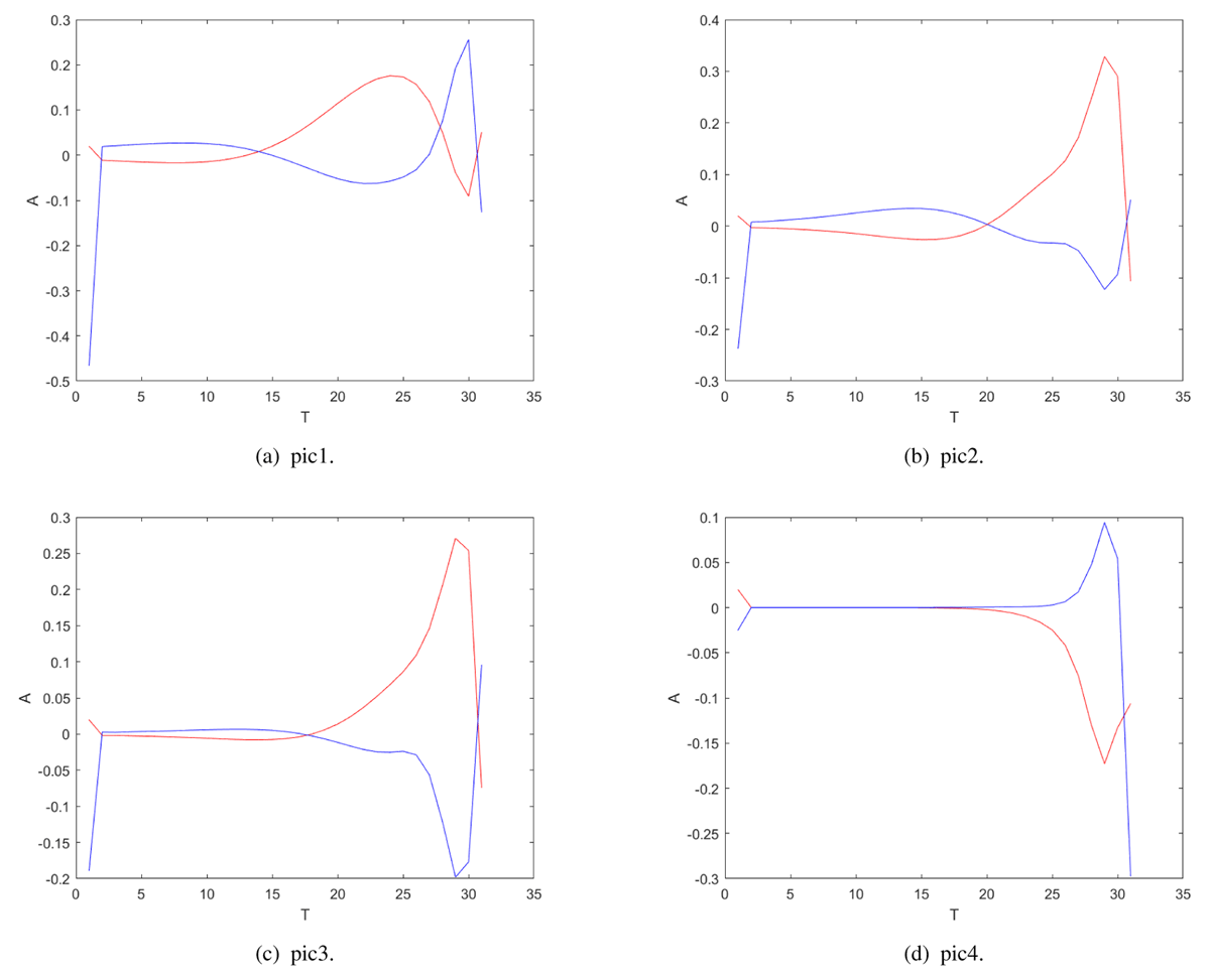
Figure 1
Ar(X) and Ai(X) dished at b = 0.4, 0.6, 0.8 and 10, respectively.
In Figure 2, it can be seen from the figure that the real part of R tends to a stable state all the time, and it does not diverge with the change of X. The β effect and zonal shear flow together inhibit the divergence behavior. When the latitude is small, the imaginary part of R has some divergent behavior. At this time, the β effect mainly plays a role of smoothing instability. However, with the increase of zonal shear flow, the β effect begins to weaken, and the chaotic behavior is completely suppressed by zonal shear flow, and the imaginary part of R is completely stable.
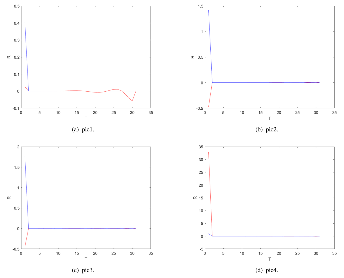
Figure 2
Rr(X) and Ri(X) dished at b = 0.4, 0.6, 0.8 and 10, respectively.
In the study of Pedlosky (2019), the influence of β effect on the development of unstable baroclinic wave was mainly studied, and it was found that β effect could reduce its instability. However, in the real atmosphere, zonal shear flow also has a certain effect on baroclinic wave instability. It can be seen from the results that the β effect has a certain influence on the baroclinic wave instability when the latitude is small, but when the latitude increases, the zonal shear flow is enhanced, and the zonal shear flow plays a leading role. The zonal shear flow can weaken the chaotic behavior, slow the change of chaotic behavior in space, and finally smooth the solution and tend to be stable.
The nature of baroclinic instability is the stability of large-scale atmospheric motion. When the wavelength of a planetary wave is larger than the critical wavelength, the wave will be unstable. Ploskoy (1987) proposed a theory of small dissipation, in which unstable baroclinic waves interact with each other and produce amplitude fluctuations. With the decrease of dissipation, the solution evolved from stable wave to periodic oscillation and finally obtained chaotic behavior at a small dissipation rate. In our study, it is found that zonal shear flow can reduce chaotic behavior. Baroclinic instability theory is the key mechanism for the generation and development of large-scale atmospheric disturbances, and common weather problems are also caused by baroclinic instability. Further research on baroclinic instability will bring impetus to the development of atmospheric dynamics and related fields.
4. Discussion
The chaotic behavior of weakly nonlinear and slightly unstable baroclinic instability is strongly influenced by the planetary β effect. In weakly nonlinear and moderately unstable systems, chaotic behavior occurs only when β is expected to be very small. When the potential vorticity gradient of β effect relative to the fundamental shear flow is insignificant, even small planetary vorticity gradients lead to dramatic smoothing of the amplitude dynamics. As β increases, chaotic behavior gives way, through a sequence of period halving, to regular steady waves (Pedlosky, 1981). When we introduce zonal shear flow, we take UB and UT are related to latitude y, we consider that the basic flow is a quadratic function of latitude. Pedlosky (2019) uses constant UB and UT, even when considering velocity profiles of the form U(1–ay2), with small a, if ay2 is ignored, then U becomes a constant, which is the same as the problem discussed in the paper of Pedlosky (2019). When U is a constant, only a special case is selected to study the effects of β effect on baroclinic instability. To ensure that the research background closer to the real atmosphere, U is a function related to latitude. The situation we consider is not to ignore the y term. Under this condition, the zonal shear flow reduces the chaotic behavior. As can be observed in our diagram, the solution is very smooth for a short period time, but as time goes on, chaos begins to emerge, forcing it to approach a constant after a while. The condition of a smooth change at the origin will, after a fixed time, at a certain distance from the origin, the amplitude will change from one feature to another. Due to the chaotic behavior along the characteristic lines in the downstream coordinate system and in the slow coordinate system, the solutions of the adjacent characteristic lines, although very close, still diverged in the first order, which led to the abrupt change of the spatial variables of the system. Entering the second derivative of zonal shear flow can eliminate chaos and smooth the solution in space. We demonstrate that zonal mean flow can modify baroclinic instability by considering the effect of zonal flow on baroclinic instability (by perfecting the related stream function).
The development of large-scale motion is usually related to the baroclinic nature of the atmosphere. Baroclinic instability theory has promoted the theoretical development of related fields, such as large-scale atmospheric stability, wave-flow interaction, and numerical weather prediction. It has confirmed that baroclinic instability theory has indeed promoted the generation and development of large-scale weather systems at middle and high latitudes. And the baroclinic instability wave theory proposed by Eady (1949) has an important guiding role in modern weather forecast. Therefore, the study of the factors affecting the development of unstable baroclinic waves is of great significance to the development of atmospheric dynamics. It is found that zonal shear flow has a non-negligible effect on atmospheric baroclinic. As the zonal shear increases, the stability of the space gradually increases. At the same time, the influence of zonal shear flow and β effect on the downstream development of baroclinic wave is considered, which makes the obtained results more comprehensive. However, there are many factors that affect baroclinic, and we need to further in-depth study and continue to advance and improve in future work.
Appendices
Appendix
Detailed derivation of the perturbation streamfunctions ϕB and ϕT equations
This appendix we derive the equation (2.3) in detail. The barotropic and baroclinic steamfunctions
where
When n = 1, 2 Eq. (2.1)
We insert Eqs. (A.1) into Eq. (A.3) to obtain the perturbation streamfunctions ϕB, ϕT, respectively,
Eq. (A.4a) and Eq. (A.4b) are added and subtracted respectively
In Eqs.
(Matthew Spydeil and Paola Cessi, 2003; Meng Lu, Lv Ke-li, 2002), where i = B, T. Therefore, Eqs. (A.5) can be reduced to Eqs. (2.3).
Acknowledgements
The work is supported by the National Natural Science Foundation of China (Grant No.42275052,12262025), Development plan of young scientific and technological talents in Colleges and Universities in Inner Mongolia (Grant No. NMGIRT2208) and the Basic Science Research Fund in the Universities Directly Under the Inner Mongolia Autonomous Region (Grant No. JY20220331), Key Scientific Research Projects of Colleges and Universities in Inner Mongolia Autonomous Region (Grant No. NJZZ23087).
Competing Interests
The authors have no competing interests to declare.