
Table 1
List of simulations. The mean horizontal resolution is given by [km] and the model top height by Ht [km]. Also listed are the grid type, whether the model is coupled to the ocean, how convection is treated, the type of boundary layer parameterisation, and whether subgrid-scale orography is parameterised. For convection, S indicates that shallow convection is parameterised and F indicates full parameterisation. No convective parameterisation is indicated by x. The types of boundary layer parameterisations include diagnostic eddy diffusivity (K), prognostic turbulent kinetic energy (TKE) or turbulent total energy (TTE), Smagorinsky scheme (S), and Simplified Higher Order Closure (SHOC).
| SIMULATION | HT | GRID | COUPLED | CONV. | BL | SSO | COMMENTS | |
|---|---|---|---|---|---|---|---|---|
| IFS-9 | 9 | 80 | Octo | yes | F | K | yes | hydrostatic |
| IFS-4 | 4.5 | 80 | Octo | yes | S | K | yes | |
| ICON-nwp | 2.5 | 75 | Icoso | no | x | TKE | no | |
| ICON-sap | 5 | 75 | Icoso | yes | x | S | no | |
| ICON-sap+ | 5 | 75 | Icoso | yes | x | S | no | continuation of ICON-sap |
| ICON-vdu | 5 | 75 | Icoso | no | x | TTE | no | |
| ICON-vdc | 5 | 75 | Icoso | yes | x | TTE | no | |
| ICON-vda | 5 | 75 | Icoso | yes | x | TTE | no | increased albedo |
| GEOS | 3 | 80 | Cube | no | F | K | yes | deep plumes disabled |
| SHiELD | 3 | 40 | Cube | mixed-layer ocean | S | TKE | yes | |
| SCREAM | 3 | 40 | Cube | no | x | SHOC | no |
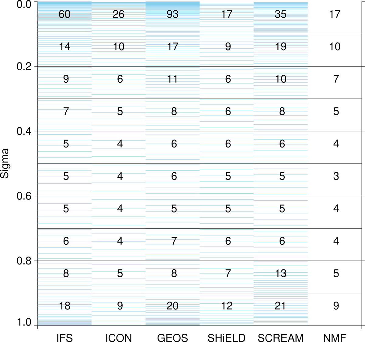
Figure 1
Vertical distribution of levels (blue lines) in the simulations of the IFS, ICON, GEOS, SHiELD and SCREAM models. Sigma is computed as the average pressure of a model level divided by the pressure at mean sea level. The number of levels falling into 0.1 wide sigma intervals is shown by numbers. The column NMF shows how the 68 sigma levels used for the normal mode function decomposition are distributed.
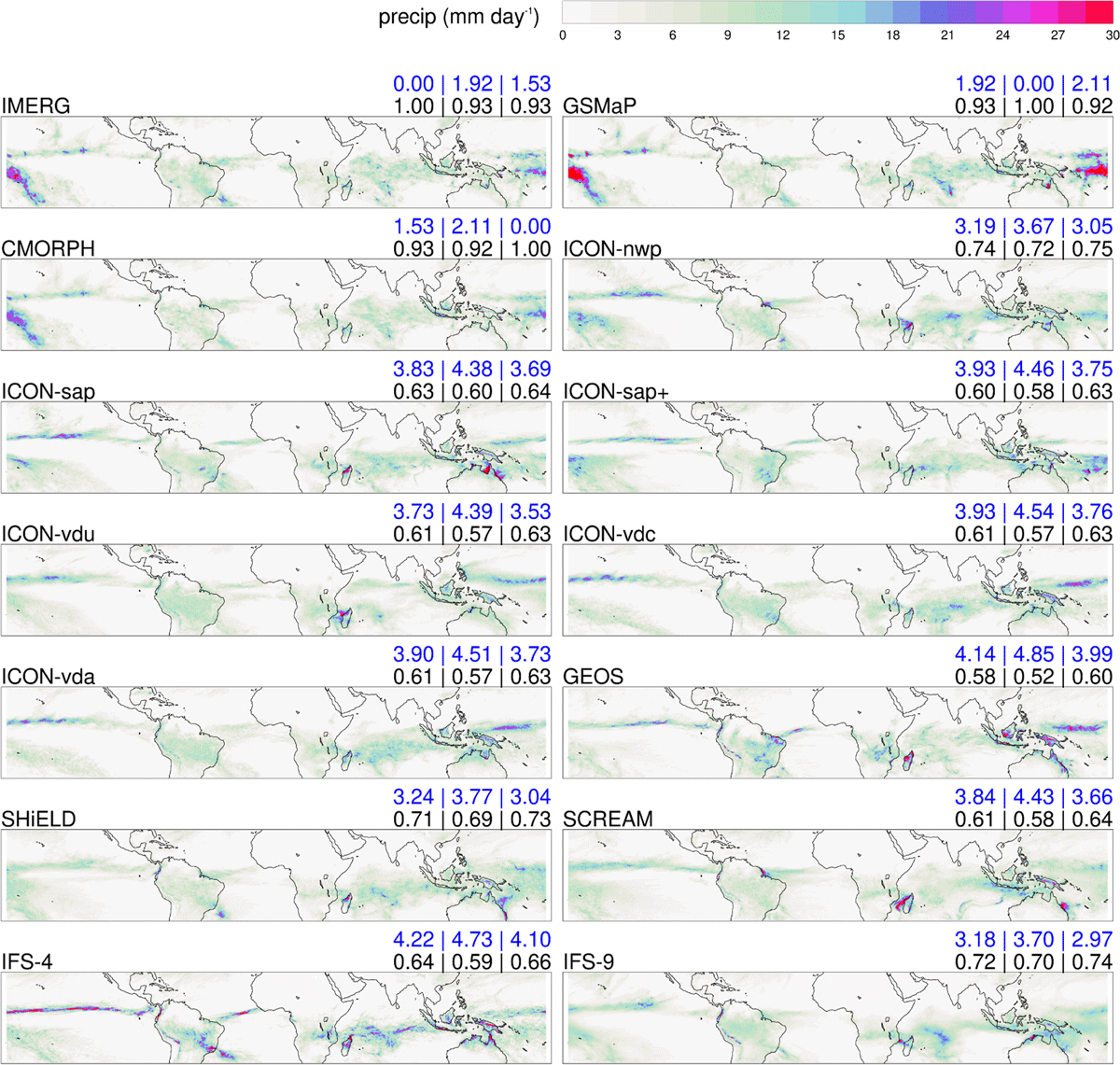
Figure 2
Forty-day mean precipitation in the tropics (30°S to 30°N). Blue numbers above the panels list the root-mean-squared errors with respect to IMERG (left), GSMaP (middle) and CMORPH (right). The black numbers list spatial linear correlation coefficients.
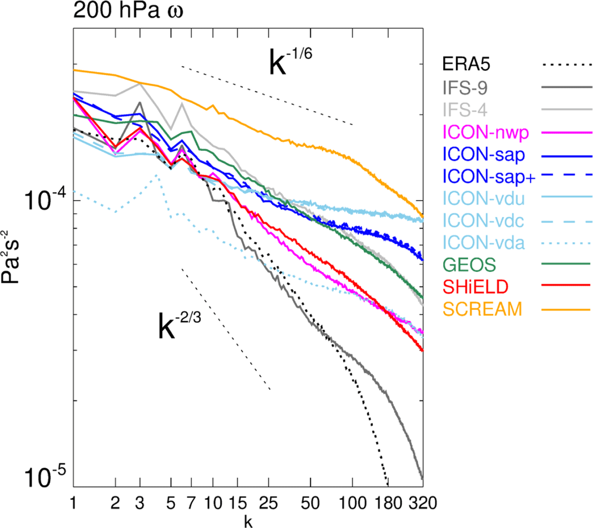
Figure 3
Tropically-averaged (30°S to 30°N) zonal-wavenumber spectra of 200 hPa pressure velocity. Dashed black lines show reference slopes.
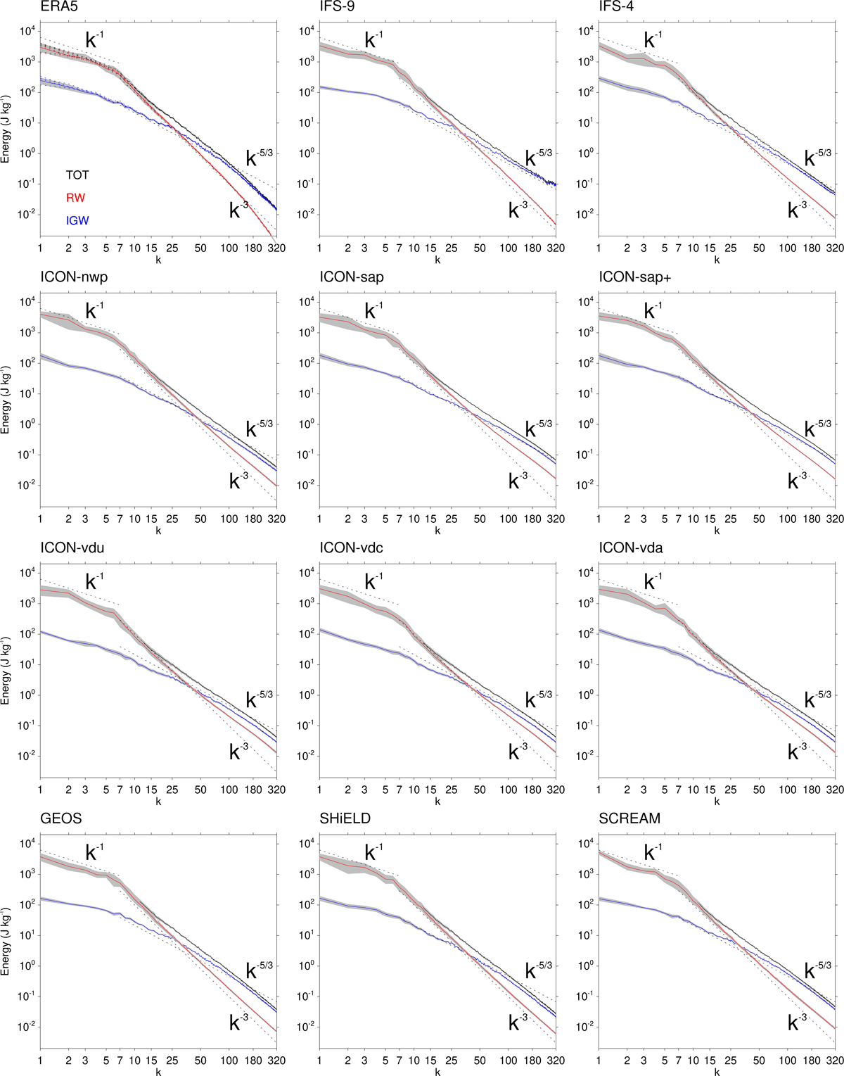
Figure 4
Global energy spectra as functions of non-dimensional zonal wavenumber k in the ERA5 reanalysis and the simulations. Shown are the total (TOT; black), RW (red), and IGW (blue) spectra. In addition to the year 2020, the ERA5 panel shows in dashed lines the corresponding spectra for 2016, 2017, 2018, 2019. Grey shading marks the standard deviation computed on 6-hourly data. For reference, spectral slopes of k–1, k–5/3 and k–3 are drawn as black dashed lines. Their locations are identical in each panel. The axis range is also identical.
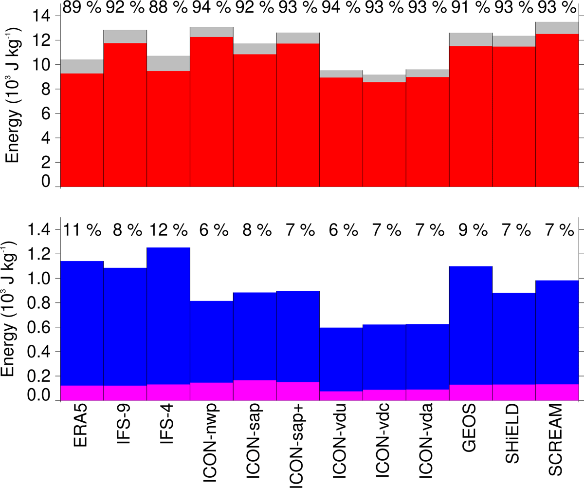
Figure 5
Total energy in the zonal wavenumbers 1–320 for the RW (red; top) and IGW (blue; bottom) modes. Grey bars on top of the red bars repeat the blue bars, such that red+grey is the total energy (TOT = RW + IGW). The percentages above each histogram show how the total energy is partitioned into RW (top) and IGW (bottom) energy (still excluding k = 0). Magenta bars in front of the IGW bars mark the IGW contribution by Kelvin waves.
Table 2
Spectral slopes in three wavenumber bands for the total (TOT), RW, and IGW modes shown in Figure 4, and the crossing scale kc. Also listed are the length scales Lc that correspond to kc. The values for Lc are computed for the equator and the midlatitudes (φ denotes latitude).
| WAVENUMBERS: | TOT | RW | IGW | Kc | Lc [km] | |||||||
|---|---|---|---|---|---|---|---|---|---|---|---|---|
| 1–7 | 8–50 | 51–320 | 1–7 | 8–50 | 51–320 | 1–7 | 8–50 | 51–320 | φ = 0 | φ = ±45° | ||
| ERA5 | –1.1 | –2.5 | –2.8 | –1.1 | –3.0 | –3.7 | –0.9 | –1.6 | –2.6 | 25 | 1601 | 1132 |
| IFS-9 | –1.0 | –2.6 | –1.9 | –1.0 | –3.1 | –3.0 | –0.6 | –1.6 | –1.7 | 32 | 1251 | 885 |
| IFS-4 | –1.1 | –2.5 | –2.2 | –1.2 | –3.0 | –2.6 | –0.9 | –1.6 | –2.1 | 24 | 1668 | 1179 |
| ICON-nwp | –1.1 | –2.6 | –2.3 | –1.1 | –3.0 | –2.6 | –0.9 | –1.6 | –2.0 | 49 | 817 | 578 |
| ICON-sap | –1.0 | –2.5 | –2.1 | –1.0 | –2.9 | –2.4 | –0.9 | –1.5 | –1.9 | 41 | 976 | 690 |
| ICON-sap+ | –1.1 | –2.5 | –2.1 | –1.1 | –2.9 | –2.4 | –0.8 | –1.5 | –1.9 | 41 | 976 | 690 |
| ICON-vdu | –1.2 | –2.4 | –2.1 | –1.2 | –2.8 | –2.4 | –0.9 | –1.5 | –2.0 | 42 | 953 | 674 |
| ICON-vdc | –1.2 | –2.5 | –2.1 | –1.2 | –2.9 | –2.4 | –0.9 | –1.5 | –2.0 | 42 | 953 | 674 |
| ICON-vda | –1.2 | –2.5 | –2.1 | –1.2 | –2.9 | –2.4 | –0.9 | –1.5 | –2.0 | 41 | 976 | 690 |
| GEOS | –1.0 | –2.6 | –2.4 | –1.0 | –3.0 | –2.8 | –0.6 | –1.6 | –2.3 | 29 | 1380 | 976 |
| SHiELD | –1.1 | –2.6 | –2.4 | –1.2 | –3.0 | –2.8 | –0.7 | –1.7 | –2.3 | 37 | 1082 | 765 |
| SCREAM | –1.2 | –2.5 | –2.3 | –1.3 | –3.0 | –2.6 | –0.7 | –1.5 | –2.1 | 32 | 1251 | 885 |
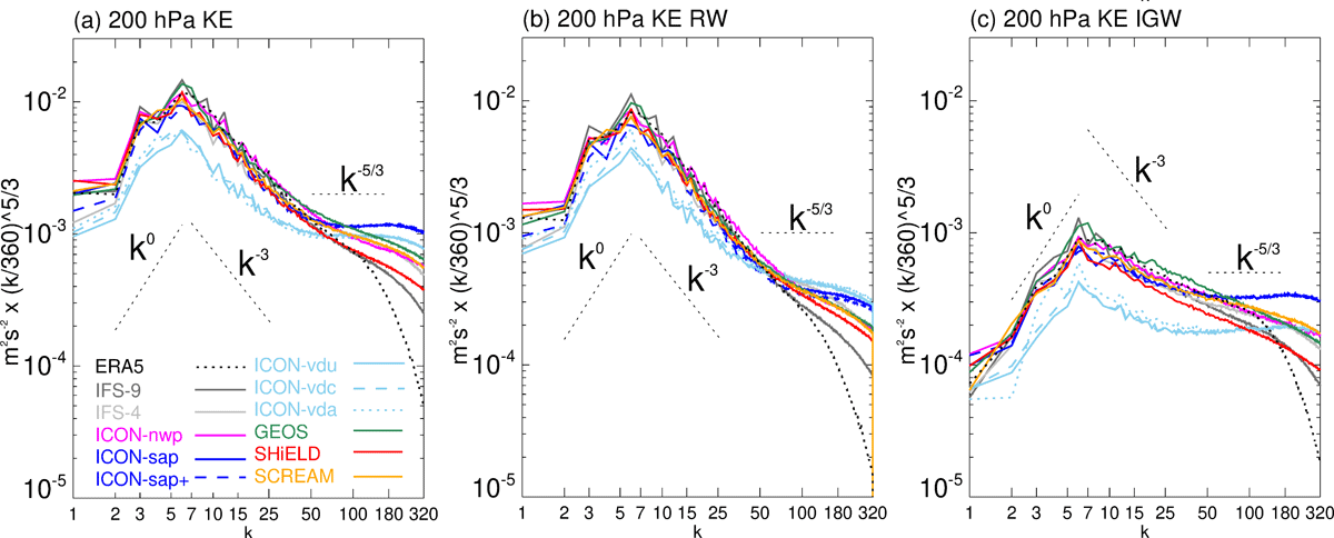
Figure 6
Compensated zonal-wavenumber spectra of tropically-averaged (30°S to 30°N) horizontal kinetic energy. Horizontal kinetic energy spectra use the (a) total horizontal wind, (b) RW circulation, (c) IGW circulation. The spectra have been multiplied by a factor of (k/360)5/3. Dashed black lines show reference slopes.
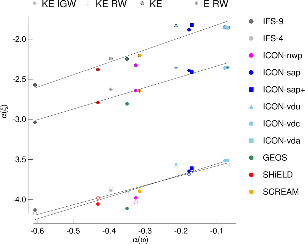
Figure 7
Relationships between spectral slopes. On the x-axis, α(ω) indicates the slope of the 200 hPa pressure velocity spectrum shown in Figure 3 for k ∈ [50,180]. On the y-axis, the slope α(ξ) is shown for four different spectra, with ξ either one of the tropical kinetic energy spectra of Figure 6 or the global RW energy spectrum of Figure 4.
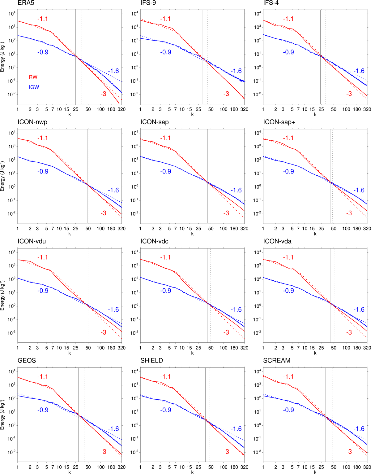
Figure 8
Sensitivity test of the crossing scale to spectral slope. The solid lines repeat the energy spectra of Figure 4. The dashed lines follow a power law kα with α constant between k = 1–7 and k = 7–320, respectively, and the values of α indicated in the panels. α is chosen as the ERA5 slopes shown in Table 2. For each simulation, the dashed curve is scaled such that the total IGW or RW, respectively, energy in k = 1–320 is not changed. The solid vertical lines mark the crossing scales of the solid red and blue curves and correspond to kc of Table 2. The dashed vertical lines indicate the crossing of the dashed curves.
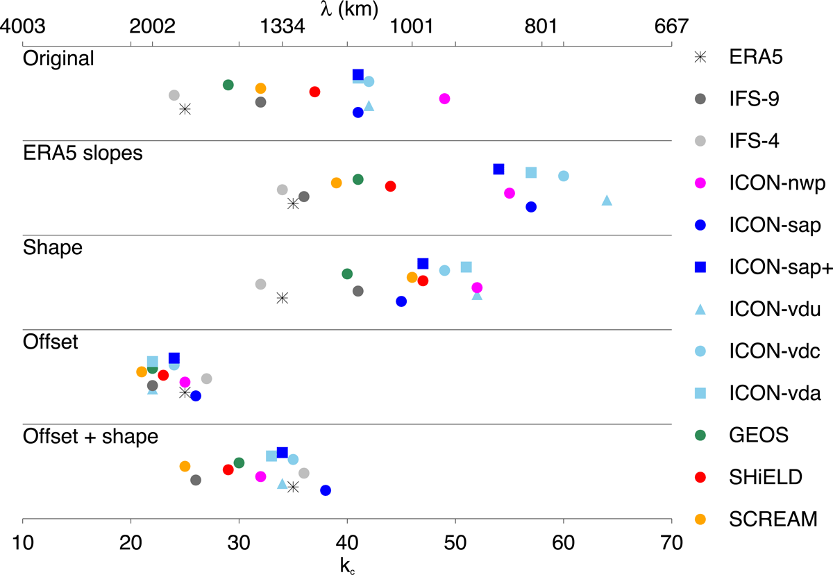
Figure 9
Original crossing scales and those of the modified spectra shown in Figure 8 and Figure 10. Symbols are vertically offset for visibility. The top row “Original” shows the crossing scales of the original spectra. The row labeled “Shape” (not shown in either Figure 8 or Figure 10) is the crossing scale that results from straightening the original spectra beyond k = 8, as done in Figure 10, but without correcting the offset. The row “ERA5 slopes” are the crossing scales marked by the dashed vertical lines in Figure 8. The row “Offset” corresponds to the magenta lines in Figure 10 and “Offset + Shape” to the black dashed vertical lines of Figure 10.
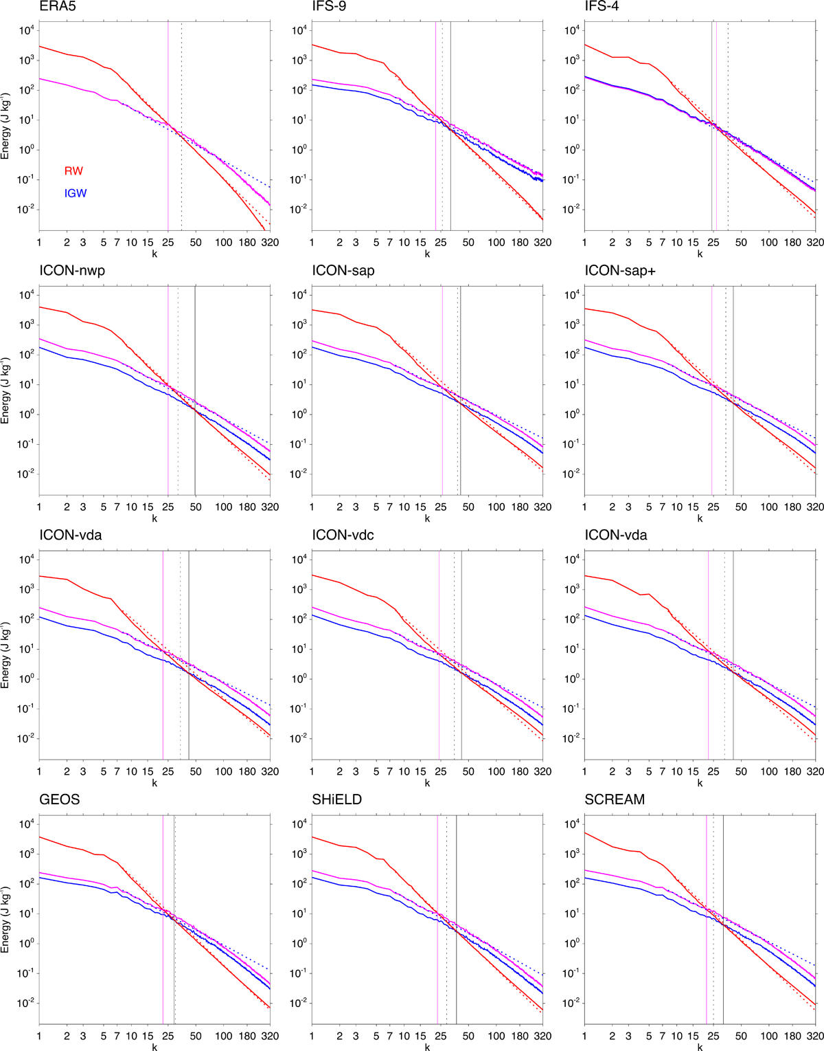
Figure 10
Sensitivity test of the crossing scale to large-scale energy offset and to shape. The solid red and blue lines repeat the RW and IGW, respectively, spectra of Figure 4. The magenta line drawn for the simulations is the IGW line offset to match the IGW/RW energy fraction at k = 1–7 of ERA5. The dashed lines continue the red and magenta lines, respectively, beyond k = 8, but with a constant spectral slope. This slope is computed from the power difference at k = 8 and k = 100. The solid black vertical lines mark the crossing scales of the solid red and blue curves and correspond to kc of Table 2. The magenta vertical lines indicate the crossing of the red and magenta lines, and the dashed black vertical lines those of the dashed lines.