
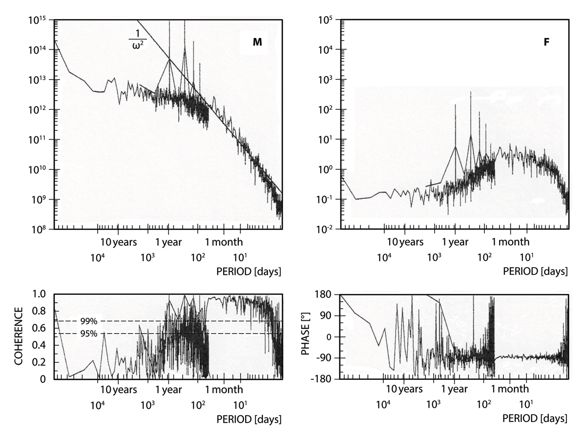
Figure 1
Spectra of the global atmospheric axial absolute angular momentum M (top left) and the global torque F (top right), and the coherence (bottom left) and phase (bottom right) spectra between M and F. The spectra (adopted from (J.-S. von Storch 1999a) consist of a high-frequency part derived from 10-year daily data and a low-frequency part derived from 500-year monthly data, produced by a coupled atmosphere-ocean GCM. A further analysis using 200-year half-daily data produces essentially the same result (not shown). Despite the strong sampling errors, the same characteristics, namely the essentially white low-frequency plateau of M, a tendency for the spectrum of F to decrease with decreasing frequency at not too low frequencies before becoming white at the lowest frequencies, the coherent 90◦-phase relation at not too low frequencies and the break-down of the coherence at the lowest frequencies, are also found for the Lorenz solution shown in Figure 7.
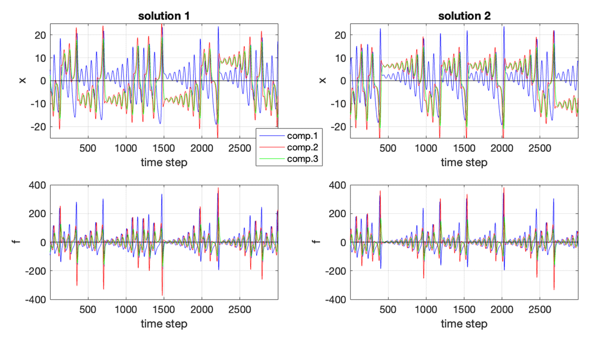
Figure 2
Pieces of two equilibrium solutions (left and right column) obtained by integrating the Lorenz system from two different initial conditions. Top panel shows the three components (green, red, blue) of the two equilibrium solutions xs and the bottom one the respective differential forcing. For each record, the respective record mean is removed. Here and in all other figures, an equilibrium solution is obtained in two steps. The first step consists of a spin-up integration, that starts from a near-equilibrium state and lasts 5 × 10³ time steps. A near-equilibrium state is a state obtained after a long integration (over 5 × 10⁵ time steps), that is then perturbed by adding a small normally distributed random variable. In the second step, an equilibrium solution is produced by integrating the model from the end state of the spin-up integration. Throughout this paper, the Lorenz model is integrated using a Runge-Kutta method with a time step of 0.01.
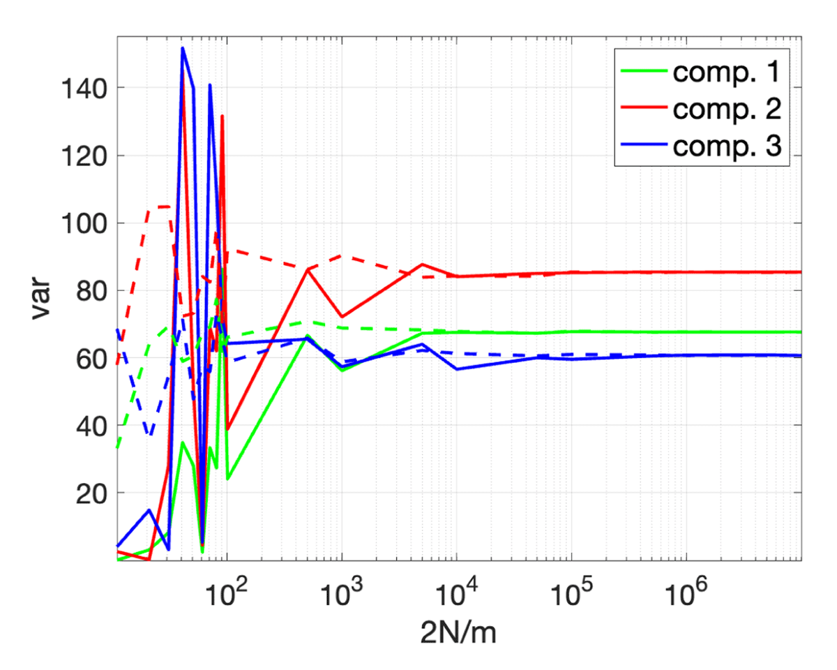
Figure 3
Variances (as defined in Eq.(9a)) obtained from a single Lorenz equilibrium solution via time average (solid) and variances Em(x2) (as defined in Eq.(9b)) obtained by averaging an ensemble of Lorenz equilibrium solutions (dashed), for the components of the 3-dimensional Lorenz state vector x (green, red, blue). Abscissa shows 2N with 2N + 1 being the length of the equilibrium solution used for time average, and m being the number of equilibrium solutions used for ensemble average.
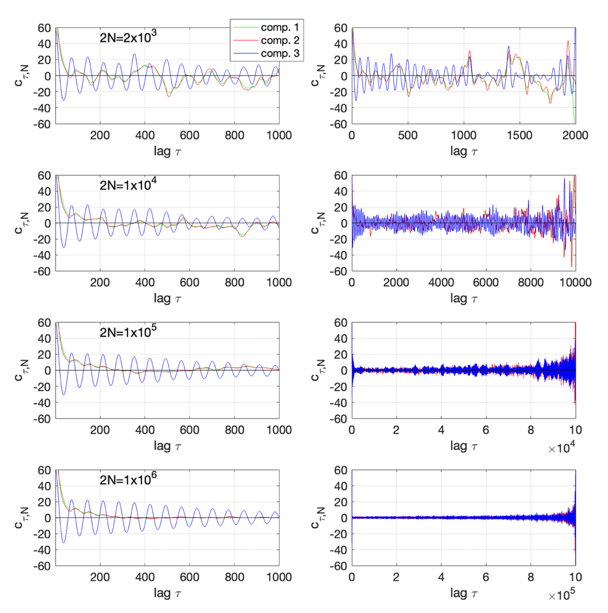
Figure 4
Auto-covariance functions cτ,N (as defined in Eq.(11)), obtained by averaging for each value of τ the two-time products xs–τxs available from a single equilibrium solution of length 2N + 1 with 2N = 2 × 10³ in the first, 2N = 104 in the second, and 2N = 105 in the third, and 2N = 106 in the last row, for the three components of the Lorenz state vector x (green, red, blue). The left column shows cτ,N at small time lags. The right column shows cτ,N at all time lags.
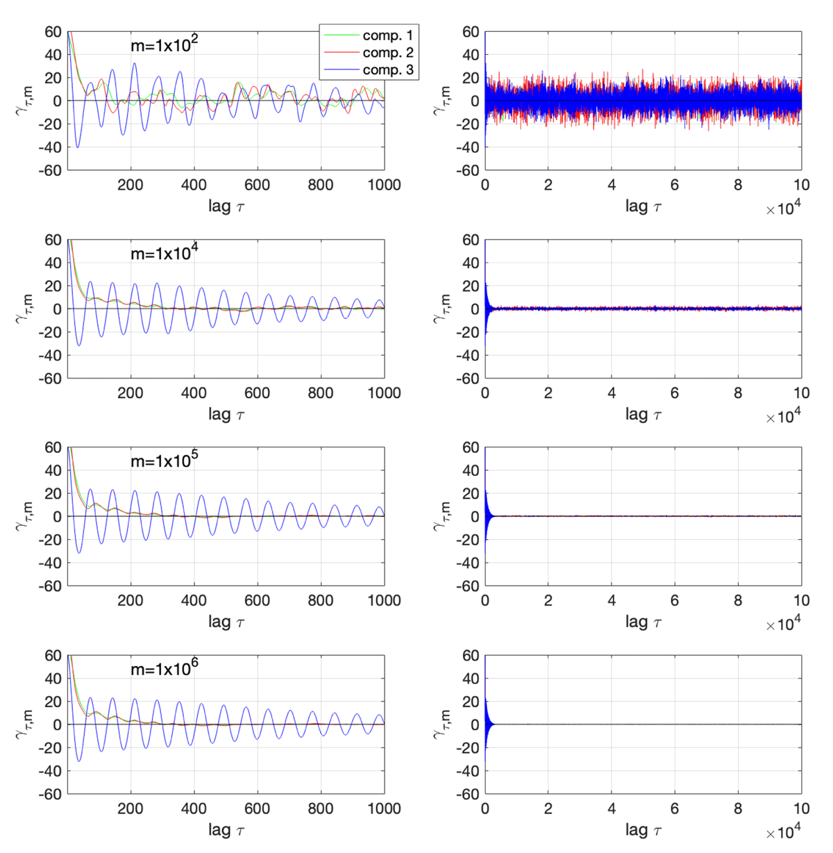
Figure 5
Auto-covariance functions γτ,m (as defined in Eq.(13)), obtained by averaging for each value of τ the two-time products xs–τxs from an ensemble of equilibrium solutions with the ensemble size being m = 102 in the first, m=104 in the second, m = 105 in the third, and m = 106 in the last row, for the three components of the Lorenz state vector x (green, red, blue). The left column shows γτ,m at small time lags. The right column shows γτ,m at all time lags.
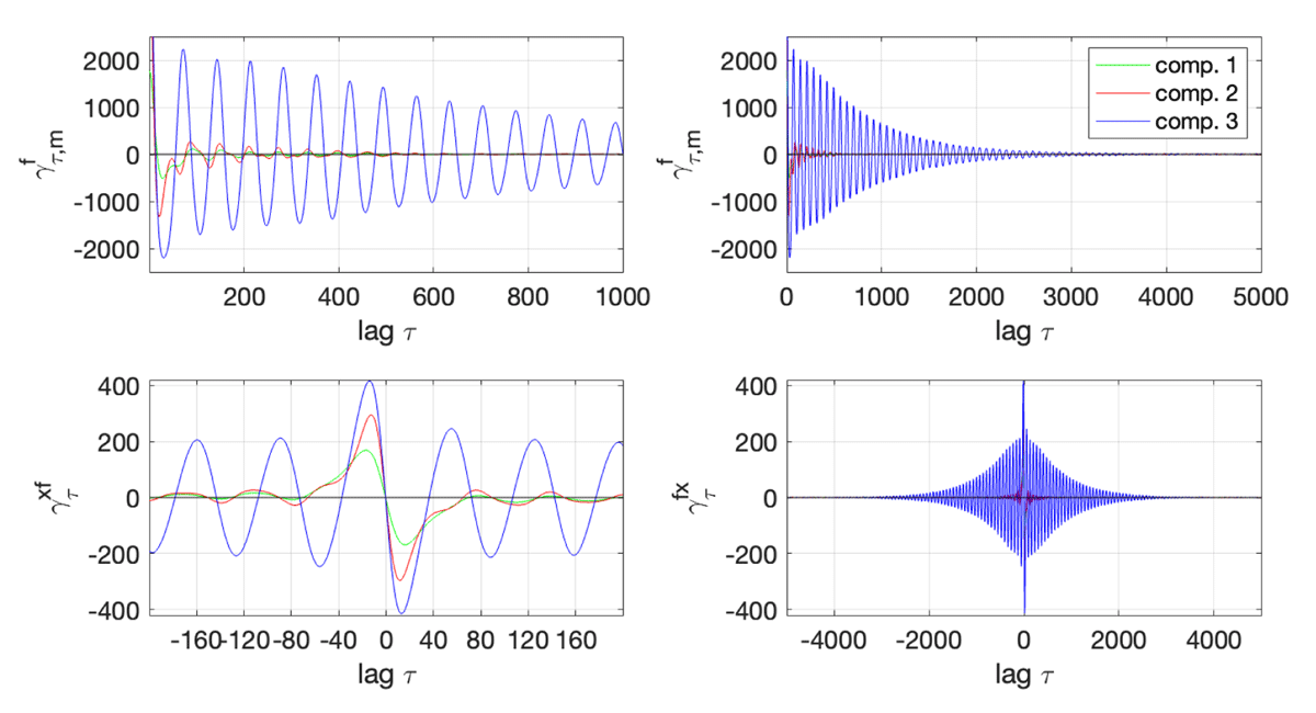
Figure 6
Auto-covariance functions of differential forcing f of component x (top), and cross-covariance functions between x and f (bottom), estimated as and following Eq.(13), for the three Lorenz components (green, red, blue). The left column shows these functions at short time lags; whereas the right column shows them at all considered time lags. is calculated using x and f of the same equilibrium solution. The average Em(·) is performed for an ensemble of size m = 106. Note that the cross-covariance function is not exactly anti-symmetric according to Eq.(24).
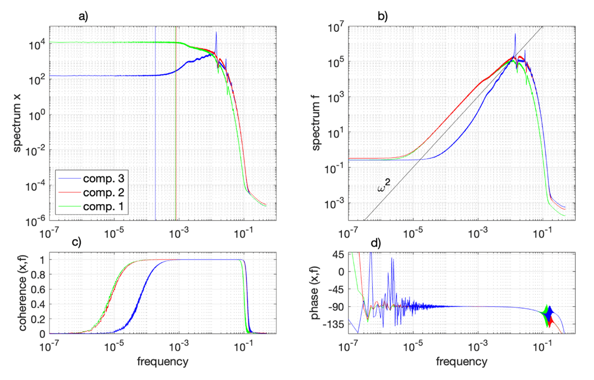
Figure 7
Spectra of component x (top left), spectra of the differential forcing f of x (top right), coherence (bottom left) and phase (bottom right) spectra between x and f for the Lorenz components (green, red, and blue). All spectra are derived as the average of m = 1000 sample spectra or sample cross-spectra, each derived from an equilibrium solution of length 2N = 107. A sample cross-spectrum is derived from x and f obtained from the same equilibrium solution. Following Eq.(B5), the sample spectra of x and f are defined as and , and the sample cross-spectrum between x and f is defined as , where and are, respectively, the Fourier coefficients used to Fourier decompose finite records of x and f. The ensemble averaged cross-spectra is used to obtain the coherence and phase spectrum between x and f, following the usual definition of these spectra. The colored vertical lines, which are considered in Section 6, indicate the frequency ω* at which the spectrum of x starts to deviate more than 5% from its low-frequency plateau. ω* is determined from running averaging the spectra shown in a) to further reduce the remaining sample variations.
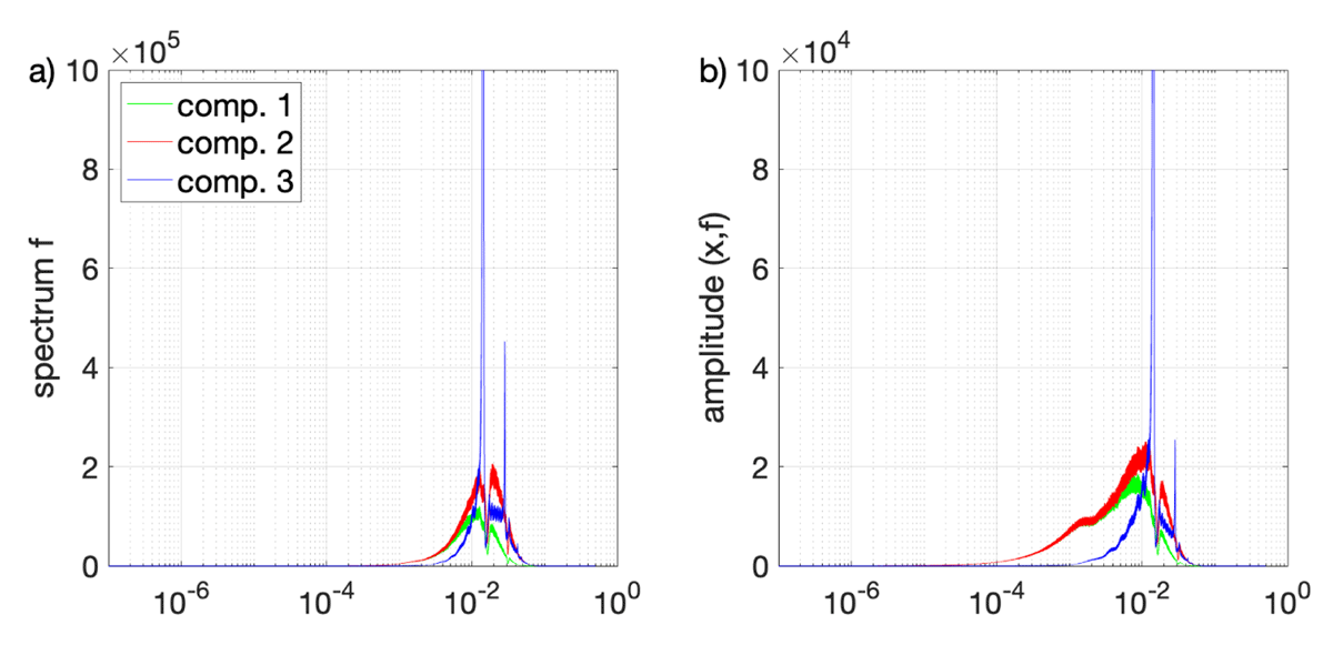
Figure 8
Γf (same as in Figure 7b) and amplitude spectrum Axf(ω) between component x and its differential forcing f for the Lorenz components (green, red, blue), estimated as in Figure 7, but plotted in linear scale.
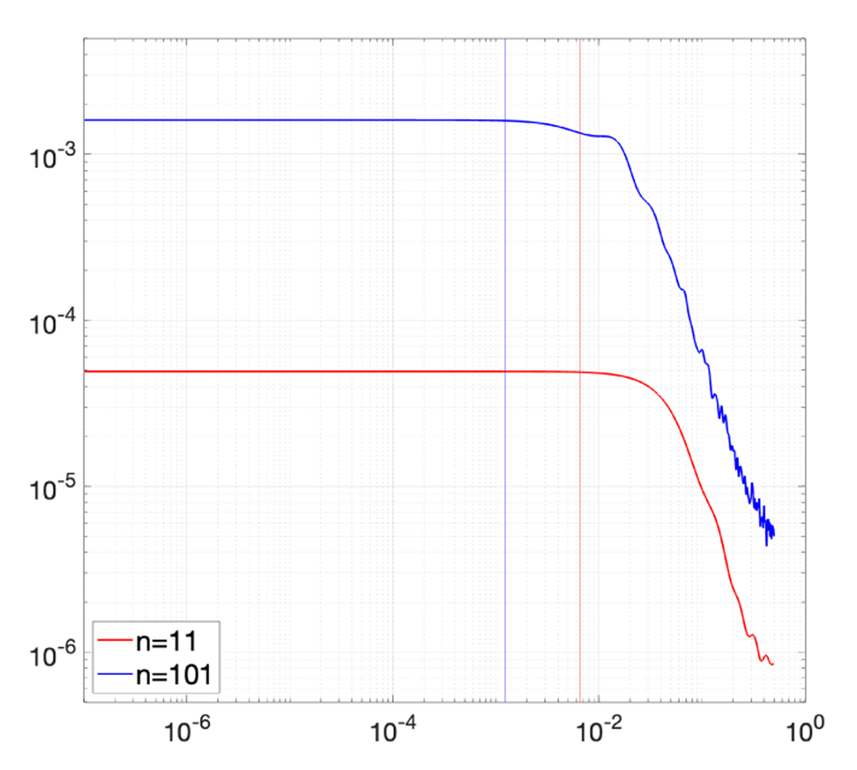
Figure 9
Spectra of two impulse-like signals of length 1 × 10⁷ + 1. The signals are not zero at the central n = 11 (red) and n = 101 (blue) time steps, but zero at other 1 × 10⁷ + 1 – n time steps. The values of the signal at the central n time steps are obtained from an AR1-process with the AR1 coefficient being 0.9. The spectra shown are averages over 100 sample spectra obtained from 100 similarly generated impulse-like signals. The spectra are white and non-zero over the low-frequency interval [0,ωs], with ωs (vertical lines) being dependent on n. The smaller the value of n, the larger the frequency ωs, the wider the interval [0,ωs]. As n → 1, the spectrum of an impulse-like signal approaches the spectrum of a delta function, which is white and equals the lag-zero auto-covariance (the only non-zero value of the auto-covariance function) at all frequencies according to Eq.(14). This n-dependent spectral behavior is independent of the details of the AR1-process used to produce the non-zero values of the impulse-like signal at the central n time steps. ωs is identified as the frequency at which the spectrum deviates 1% from its value at the lowest resolved frequency.