
1. Introduction
Rainfall is one of the major and important environmental parameters which is responsible for floods, droughts, and drastic events like land sliding. The drastic floods of 2009 and 2010 caused more than 43 billion USD to Pakistan’s total economy and more than 178 causalities (see.,https://en.wikipedia.org/wiki/2010_Pakistan_floods). However, Kirsch et al. (2010), claimed the 1700 casualties and 9.743$ billion known loss to local infrastructure, which includes school, healthcare units and some other government institutes. Therefore, there is a great need to predict rainfall variables more precisely. Pakistan monitoring stations are not equally distributed across the country. In the north of Pakistan, episodes of heavy rainfall are prevalent. However, there are very few monitoring stations in this area. On the other hand, a large number of monitoring stations are deployed in the southern region fewer episodes of rainfall are recorded there.
There is an impulse need to revisit the distribution of the monitoring network of the rainfall. This can potentially be done by removing redundant locations from the existing monitoring network. Further, new monitoring stations can be deployed to predict the environmental parameters more precisely. Adding optimal and deleting the redundant locations can reduce prediction errors.
Modelling the spatial behavior of different environmental parameters has been studied by many researchers (Hengl et al. 2004, 2007; Ikechukwu et al. 2017; and Yang, 2018). Geostatistical models provide flexible approaches to capture the spatial behavior of the environmental parameters. Spatial prediction or Kriging techniques belongs to a family of geostatistical techniques, that mainly focus to investigate the spatial behavior of the data. Kriging procedures have been widely used for spatial prediction of the environmental parameters, groundwater, droughts, and soil sample prediction at different locations. Zahid et al. (2016) modeled the spatial distribution of the sodium concentration by means of Universal Kriging and Bayesian Universal Kriging in groundwater. It was found that Bayesian Universal Kriging better-fitted the data.
Spatial prediction of sulfate concentration in groundwater has been carried out for the Southern Punjab of Pakistan (Mubarak et al. 2015). A study on mapping and spatial prediction of the average annual precipitation of Turkey by using the five different kriging methods has been carried out by Bostan et al. (2012). The rainfall on 225 meteorological stations was measured and the superiority of universal kriging was showcased. Many simple and complex interpolation methods have been developed to estimate the value of spatially distributed data including the environmental parameters at unobserved locations on the basis of observed location (see the massive literature e.g. Knotters et al. 1995; Phillips et al. 1997; Carrera-Hernández and Gaskin, 2007; Wang et al. 2002; Wang et al. 2010; Hussain et al. 2014; Omer et al. 2019; and Ellahi et al. 2021).
Modelling the spatial distribution and characteristics of the particular matter remains a focal point of research. There are numerous optimisation methods to identify the optimal solution for any monitoring network. Spatial sampling design is widely used to identify the optimal solution for the monitoring network (see the recent massive literature, e.g., Fuentes et al. 2007; Zhu and Stein, 2006; Zimmerman 2006, Spöck and Pilz, 2010; Hussain et al. 2010; Hussain et al. 2011; Hussain et al. 2015 and Khan et al. 2021). The optimal spatial sampling designs can provide minimum mean square prediction error. The resultant optimized monitoring networks can save cost of installation and manpower. Despite being widely used, spatial sampling design is one of the topics that could not get enough attention in the literature due to laborious and complex mathematical computations. Unfortunately, sometimes the spatial sampling design failed to produce reliable results. In such cases, stochastic search algorithms (Guedes et al. 2011) are used. The stochastic search algorithm has been extensively used in spatial statistics to find the optimal solution for the different monitoring networks (see e.g., Journel, 1990; Deutsch and Cockerham, 1994; Gringarten and Deutsch, 1999; Al-Mudhafar, 2019). The choice of stochastic search algorithms is typically based on how the algorithm deal with arbitrary systems, statistical guarantees for finding an optimal solution, computational cost, and accuracy The Spatial Simulated Annealing (SSA) has many features of a good search algorithm. Similarly, a Genetic Algorithm (GA) can end up with multiple local optima. It is a global optimization method that can provide a good solution by utilizing the minimum available information. Also, it provides a good and fast convergence towards an optimal solution (Gallagher and Sambridge, 1994). Gallagher and Sambridge (1994) discussed two stochastic search algorithms (GA and SSA). SSA and GA has widely been used to optimize the monitoring network of the rainfall distribution. Pardo-Igúzquiza (1998) established an optimal network design to estimate the areal averages of rainfall events by using the SSA. Recently, Wadoux et al. (2017) utilized the SSA to minimize the space-time average kriging external drift variable to find an optimal solution for the monitoring network of the rainfall network in the north-east of the city of Manchester in the United Kingdom. Adib and Moslemzadah (2016) presented the optimal selection of the rainfall gauging stations by combining the kriging and genetic algorithm methods. The estimation error of different rainfall gauging estimations was calculated using inside and outside stations of the watershed. Each combination is further given to GA to select the optimal location by minimizing the error variance. More latest literature on SSA and GA to optimize the rainfall monitoring network can be visited (e.g. Nasseri et al. 2008; Soroush & Abedini, 2019; Molla et al. 2022). The next paragraph explains some of the transition histories of GA and SSA in different ways.
The GA’s and genetic programming approaches have been the most widely used in credit scoring applications. Goldberg (1975) discussed that GA provides a method to perform a randomized global search in a solution space. Metropolis et al. (1953) introduced a stochastic search relaxation method that can simulate the performance of a system of particles approaching thermal equilibrium. The algorithm compares the energy with some given criteria of different particles to that of a dissimilar algorithm. If the energy of the new configuration is smaller as compared to the previous one, the new formulation is accepted. Fabian (1997) studied the performance of simulated annealing procedures for searching a global minimum of a function. Bélisle (1992) discussed the convergence properties of simulated annealing procedures for continuous functions. These results were applied to hit-and-run algorithms used in global optimization. Fleischer (1996) introduced cybernetic optimization by simulated annealing as a procedure of parallel processing that reduced the processing time for the convergence of simulated annealing to the global optima. Furthermore, Fleischer (1999) extended the theory of cybernetic optimization by simulated annealing into the continuous domain by applying probabilistic feedback control to the generation of candidate solutions. Heuvelink et al. (2010) used the plume simulation to optimize some additional cities by minimizing the predictable cost of a wrong decision and area of false positive and false negative detection. However, this method is very time-consuming, due to geo-statistical simulation which is based on the iterative numerical optimization algorithm.
In this article, we applied the SSA and GA following the ethos of Baume et al. (2011) and Santacruz et al. (2014). Here, the Average Kriging Variance (AKV) for Pakistan Monitoring network to the rainfall distribution is minimized. Two interpolation techniques named model based OK and model based UK are being used to observe the unknown location based on known locations. The novel contribution of this article is that we modified the SSA and GA by using the model based OK and the model based UK to optimize the monitoring network of rainfall distribution in Pakistan.
This paper is distributed in six sections in total. Section 2 represents the detailed description of the data set that has been used for this research. SSA optimization technique with the model based OK and the UK is described in Section 3. Section 4 briefly explains the GA optimization technique. The results and discussion are provided in Section 5. In the end, some concluding remarks have been given in section 6.
2. Pakistan Rainfall Data Set
Pakistan is situated between 23°–37° towards north latitude and 61°–76° towards east longitude. Pakistan holds the deserts in western areas. These areas are observed to have high temperatures and remain dry. The warm season and little precipitation are observed throughout the year in the coastal areas which are situated along the Arabian Sea. The northern areas of Pakistan have mountains. The well-known Karakorum region is also in the north of Pakistan, having the world’s largest mountains. These areas are generally very cold with frequent episodes of heavy rainfall. The area between the latitude 24°–30° and longitude 62°–67° is the east-south region of Pakistan. The east-south regions have deserts. This region has low height (less than 150 m) and remains quite hot even in the monsoon period. Pakistan capital Islamabad is located between latitude 32°–35° and longitude 68°–72°. There is usually very heavy rainfall throughout the year in the capital of Pakistan. The areas with heavy rainfall are above thousand-meter on average. The average elevation is 1400 m in the northern areas of Pakistan and these areas remain cold compared to all other regions of Pakistan.
In general, summer season is wet, however the winter remains dry. The average rainfall varies from 200 mm in the north to 30 mm in south.
Pakistan meteorological department is observing environmental variables at more than 90 monitoring stations. The rainfall data are collected from 52 stations from the Pakistan Meteorological Department, Islamabad, from 1998 to 2019. The aim is to cover most of the country, for which fifty-two meteorological stations are sufficient to obtain optimum results. Rainfall is considered as the most responsible environmental parameter for climate change. Pakistan’s climate is diverse. Rainfall contributes to natural disasters like floods and land sliding issues. Therefore, modelling the variation in rainfall can help in future planning. For computational ease, the monthly average rainfall is used as the response variable. We use two different optimization techniques. These were used to optimally add and delete 5, 10, 15, 20, 25 and 30 number of locations selected registered cities and from existing monitoring network, respectively.
The study area and existing monitoring network is displayed in Figure 1 above with the layers of average rainfall. On the other hand, Figure 2 shows the study area map consisting of 441 registered cities in Pakistan. from where optimal locations can be chosen from these.
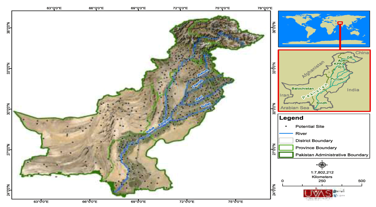
Figure 1
Study area with 441 potential candidates.
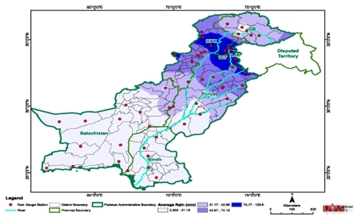
Figure 2
The 52 sampling locations in the existing rainfall monitoring network of Pakistan.
3. Spatial Simulated Annealing (SSA)
The core idea of SSA is to select new locations based on some performance criteria. We modified the SSA by minimizing AKV of the model based on OK and UK, following the ethos of Riberio and Diggle (2007). It starts with the initial design and computation of the objective function AKV. Then, it produces a new design by moving one randomly chosen point from some random direction. Again, compute the objective function for the new design. Accept the new design with some probability if the objective function is improved. Decrease the probability by increasing the iterations of algorithms. Repeat these steps until the objective is met. It was noted that accuracy increased as we increased the number of iterations of the process. In this study, 10,000 iterations were carried out for achieving the objective. Spatial Simulated Annealing needs some other parameters to be defined as well. For instance, the probability of accepting and rejecting the new design, ‘Colling’ schedule and a stopping criterion are also required for achieving the underlying objective. The two well-known interpolation procedures OK and UK with known variogram models are used for simulated annealing. The next two subsections give the detailed description of the used interpolation procedures.
3.1. Model Based Ordinary Kriging
Let Z(s1), Z(s2) Z(s3), ….., z(sn) be random variables at spatial locations s1, s2, s3, …., Kriging is an interpolation technique used to predict the unknown values of a random variable, Z, at one or more unobserved locations, stating differently, kriging is used to interpolate random field, Z, at unobserved locations (Matheron, 1963). The South African engineer D.G. Krige is the pioneer founder of kriging and this technique was named on his name. The main developments came in kriging from G. Metheron after 1960. So far numerous kriging techniques have been developed like Ordinary kriging (OK), Universal Kriging (UK), Simple Kriging (SK), Regression Kriging (RK), Bayesian Kriging (BK), and many more can be found in the literature. One of the major benefits of this technique is that it calculates the prediction error of the response variable. Kriging considers the spatial dependence for mapping purposes, and also for sampling locations. The spatial dependence is further modelled by fitting theoretical variogram model to empirical variogram. The variogram model can be written as
Where Z(si) and Z(sj) are the realizations of the response variable at known locations si and sj respectively, and N(h) is the number of point pairs falling within the distance h (Riberio and Diggle, 2007). OK is one of the efficient techniques which has been used frequently. The basic assumption of this technique is that the mean is considered constant but unknown. This technique has the ability to produce the predicted values and the corresponding prediction errors. This method is believed to consider one of the simple and popular methods in spatial prediction. The response variable Z follows the Gaussian distribution in the model (see details., Riberio and Diggle, 2007). Further details could be found in
where µ is the mean and ∑z is the covariance matrix and can be written as
where R is a correlation matrix and it depends on vector-valued parameter α, (σ2 = sill; φ = range, and τ2 = nugget). Generally, Kriging techniques require the data to be normally distributed. The parameters of model can be estimated by using well-known estimation methods e.g., Restricted Maximum Likelihood (REML), Weighted Least Square (WLS), Ordinary Least Square (OLS), and Maximum Likelihood (ML).
The variogram model which produces minimum Mean Square Prediction Error (MSPE) is preferred for interpolation of the response variable. The response variable at the unobserved sites can be predicted by the system of ordinary kriging as follows.
where wi are the weights to fulfil the condition of unbiasedness.
The Lagrange multiplier can be used to minimize the variation of prediction subject to unbiasedness.
3.2. Model Based Universal Kriging (UK)
A process that offers an estimator including the local trend in the data set is known as Universal Kriging (Isaaks and Srivastava, 1989). In the previous subsection, it is illustrated that in OK, mean remain constant but unknown in whole study area, however in UK, the mean is the function of some local trend’s coordinates. Mathematically model of UK can be written as follows
where µ(s) is considered as mean and ∑z is known as covariance matrix.
where R is a correlation matrix and it depends on vector-valued parameter α, (σ2 = sill; φ = range, and τ2 = nugget). The parameter estimation methods are same which have been used in OK method. The trend component in UK can be modelled as
where bk is the kth coefficient, pk is the function that defines the trend, and l is the number of functions that is used to model the trend. The remaining process for estimating the weights is similar as given in subsection (3.1).
3.3. Cross-Validation statistics
Cross-validation statistics are used to compare the performance of kriging methods (Mubarak et al. 2015). Three different methods are frequently used in the literature. These methods are named, Mean Bias Error (MBE), Mean Absolute Error (AE), and MSPE and that are as follows:
where is the estimated value of data, z(xi) is the observed value of the data. Here, MSPE is used as criterion to compare the performances of both used interpolation techniques.
4. Genetic Algorithm (GA)
Genetic algorithm (GA) deals population of string which demonstrates the parametrization of the optimization problem. In biological sense, the strings are known as genotype or chromosomes. The actual situation is to map the representation of phenotype. GA includes the characteristic to encourage/discourage the overachieving /under achieving of the string in the population. In this article, we use GA to minimizee the AKV as the interpolation accuracy measure. Interpolation procedures are already discussed in section 3.1 and section 3.2. The basic algorithm of GA at first step is to determine and define an initial population, and set k = 0. Second step, calculate the objective function that is called “fitness” function for every fellow of the population, and allocate probabilities pi to each item in the population, feasibly proportional to its fitness. Third step, select a probability sample of size m ≤ n. This is the reproducing population. Fourth step, randomly from a new population from the reproducing population, using numerous mutation and recombination rules. This can be done using random sample selection of the rule for each single pair of individuals. Fifth step, if convergence criteria are meet, stop, and convey as the optimum; otherwise, set k = k + 1 and repeat the procedure from step one.
Few of the main advantages of using the GA is, the GA has ability to solve every optimization problem, and it can solve problems with multiple solutions. GA techniques doesn’t demand the complex mathematical knowledge, and is very easy to implement and understand. The GA is used to point out optimum sites out of the n locations. Pakistan Monitoring rainfall data set of 52 network locations with their respective coordinates is used for the optimization purposes. We add and delete 5, 10, 15, 20, 25 and 30 number of new locations from existing and 441 registered cities of Pakistan, respectively, by minimizing the AKV. The AKV is calculated as
where is the Kriging variance and n is the number of samples. For evaluation of the GA, the population size is defined as 40 individuals, which means that for every n point in the network, there is 40 pairs of coordinates for each iteration. We take 10000 iterations for addition of our required points that are mentioned above.
5. Results and Discussion
This section demonstrates the twofold benefits of the of stochastic search algorithms. First, we can save the sampling locations for precise prediction; second; the accurate prediction of the rainfall parameter can be attained with fewer sampling location. In more details, visualization of 52 monitoring station from the original rainfall monitoring network is shown in Figure 1. In Figure 2, we visualize the study area along with additional 441 potential candidates from where we can add the new locations which may be used for improving the original monitoring network of rainfall. We have denser original rainfall monitoring network in the north compared to south. Therefore, the first target is to eliminate the redundant locations from the north of network. In the 2nd step, we add these locations in into the reduced network in an optimal way so that the new design should be space filling and better covering location in the south as well. We used the minimization of AKV given in equation (5) as design criteria for selecting the new locations from the 441 potential candidates. The spatial variability of rainfall is modeled between known and unknown location by Matheron variogram model (Matheron, 1989). After fitting the variogram model, we found the parameters initial range and spatial sill 8 and 2, respectively. We can consider different techniques to estimate the parameters of Variogram model, but we stick to maximum likelihood (ML) and utilize it to estimate the parameters of variogram model. The estimated nugget and partial sill are 0.2632 and 2.5324, respectively. After estimation of Variogram models parameters, we can say that it shows strong dependencies among the known and unknown locations align with the similar results Zahid et al. (2016). At second step, we made a spatial prediction of rainfall by using the model-based OK and model-based UK on 441 unobserved locations. Mean square prediction error (MSPE) is used as cross validation criteria. Observed MSPE of OK and UK is 39.64 and 37.88, respectively. The MSPE of UK is slightly lower as compared to the OK, which indicates the superiority of UK over OK.
After first two steps, we are ready to design an optimal monitoring network of rainfall distribution. We use the SSA and GA for minimizing the AKV to remove the redundant (5, 10, 15, 20, 25 and 30) locations from the existing monitoring network. We notice that most of the redundant location exists in north side as the monitoring network is denser in north (may be locations are nearer to each other). We predicted the MSPE on the reduced monitoring network and we notice a slight increase in MSPE of OK and UK, from 39.64 to 41.37, 37.88 to 39.34, respectively, while predicting the unobserved locations. Our results are pretty much aligned with the results of (Spöck and Hussain, 2012) spatial sampling design for Pakistan. We produce the visualization reduced design by removing the 30 redundant locations from existing monitoring network in Figures 3, and 4. We have the name and coordinates of the reduced design with their visualizations (can be provided on the demand). At second step, we added the (5, 10, 15, 20, 25 and 30) location in existing network of rainfall and reduced monitoring network. These new added/deleted location with SSA and GA are shown in Figures 3 and 4. Now we have multiple reduced optimal networks so we can make a spatial prediction on the reduced optimal network to check the optimality of our method. We have reduced design with 22 locations (after removing the 30 redundant location) and we add the 30 new locations those are optimally selected by the SSA and GA. We made the prediction of rainfall on 441 unobserved locations with UK and OK for the optimal added points of SSA and GA. We find a significant decrease in MSPE of UK and OK, in both cases either we add the points by SSA and GA. The MSPE of the OK and UK are recorded to 34.39 and 32.56, respectively, by considering the SSA optimal points. Similarly, The MSPE of the OK and UK are recorded 36.01 and 33.92, respectively, by considering the GA optimal points. At this stage, we can add some more remarks on the resulting optimal monitoring network of rainfall.
At first the optimal points are selected in the areas where it looks unfilled, for instance, in our case it looks empty in south. This is obvious that the kriging variance is generally more increased there. This remark is consistent with the finding of Spöck and Hussain (2012).
As whole we can say that the resulting optimal monitoring network of the rainfall distribution seems to be space filling network: It is a property statement that the examined optimal monitoring network criterion is usually based on accurate prediction not how the covariance function is best estimated. The best estimation of the covariance function also requires that the new potential candidates’ sites should be very near to each other, for instance, proper estimation of the nugget effect.
Every chosen point selected only once: Our optimal selection of the candidates is based on the without replacement selection of the potential candidates. So, our optimal selection of the points fulfils the criteria, which is usually tough to attain without stochastic search algorithms.
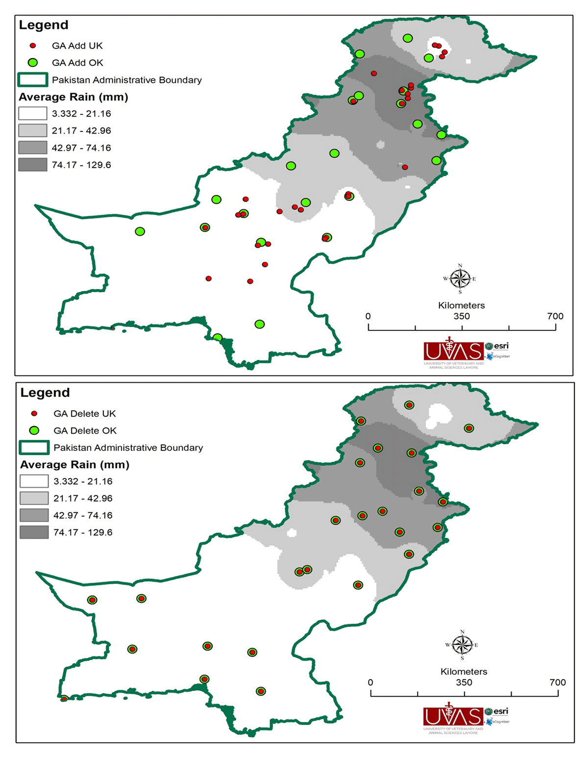
Figure 3
Geographical placement of 30 additional and deleted location by GA under both interpolation procedures for Pakistan meteorological rainfall monitoring network.
Note: Some of the points overlap each other (all the coordinate’s names can be provided on demand).
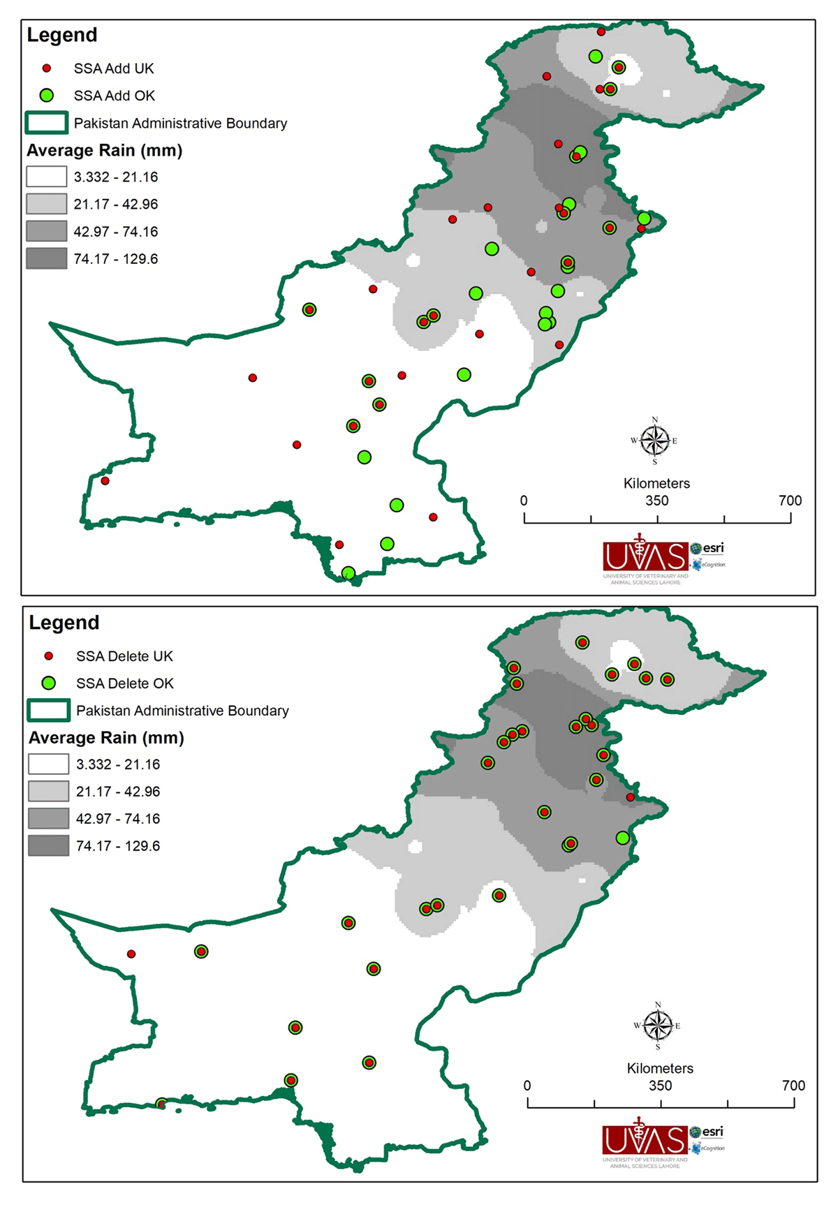
Figure 4
Geographical placement of 30 additional and deleted location by SSA under both interpolation procedures for Pakistan meteorological rainfall monitoring network.
Note: Some of the points overlap each other (all the coordinate’s names can be provided on demand).
Furthermore, Table 1 represents the AKV by using the SSA and GA to add/delete the specific number of location from/to the existing monitoring network. From the results, it can be observed that SSA remained efficient in all scenarios. We noticed that SSA and GA has less AKV with UK as prediction technique which is pretty much sure and this result is aligned to our presented cross validation results.
Table 1
Pakistan dataset: adding and deleting measurements to the initial design with OK and UK as interpolation Procedure- SA: Simulated Annealing; GA: Genetic Algorithms.
| SCENARIO | METHOD | IP | AKV | SCENARIO | METHOD | IP | AKV |
|---|---|---|---|---|---|---|---|
| Add5 | SSA | OK | 1.1498 | Del 5 | SSA | OK | 1.1935 |
| Add5 | SSA | UK | 0.8419 | Del 5 | SSA | UK | 0.9723 |
| Add5 | GA | OK | 5.0918 | Del 5 | GA | OK | 5.6001 |
| Add5 | GA | UK | 4.8221 | Del 5 | GA | UK | 5.4211 |
| Add10 | SSA | OK | 1.1181 | Del 10 | SSA | OK | 1.2070 |
| Add10 | SSA | UK | 0.8399 | Del 10 | SSA | UK | 0.9812 |
| Add10 | GA | OK | 4.9211 | Del 10 | GA | OK | 5.6821 |
| Add10 | GA | UK | 4.7811 | Del 10 | GA | UK | 5.5211 |
| Add15 | SSA | OK | 1.1181 | Del 15 | SSA | OK | 1.2286 |
| Add15 | SSA | UK | 0.8382 | Del 15 | SSA | UK | 0.9935 |
| Add15 | GA | OK | 4.8221 | Del 15 | GA | OK | 5.7211 |
| Add15 | GA | UK | 4.5211 | Del 15 | GA | UK | 5.6244 |
| Add20 | SSA | OK | 1.0943 | Del 20 | SSA | OK | 1.2563 |
| Add20 | SSA | UK | 0.8322 | Del 20 | SSA | UK | 1.0001 |
| Add20 | GA | OK | 4.7221 | Del 20 | GA | OK | 5.8001 |
| Add20 | GA | UK | 4.4321 | Del 20 | GA | UK | 5.6901 |
| Add25 | SSA | OK | 1.0832 | Del 25 | SSA | OK | 1.2955 |
| Add25 | SSA | UK | 0.8298 | Del 25 | SSA | UK | 1.0231 |
| Add25 | GA | OK | 4.6001 | Del 25 | GA | OK | 5.9211 |
| Add25 | GA | UK | 4.442 | Del 25 | GA | UK | 5.7212 |
| Add30 | SSA | OK | 1.0765 | Del 30 | SSA | OK | 1.3593 |
| Add30 | SSA | UK | 0.8923 | Del 30 | SSA | UK | 1.2322 |
| Add30 | GA | OK | 4.4211 | Del 30 | GA | OK | 5.9811 |
| Add30 | GA | UK | 5.8321 | Del 30 | GA | UK | 5.8321 |
6 Conclusion
The preceding article demonstrates the optimal monitoring network to the rainfall distribution of Pakistan that may be used quite efficiently to other monitoring network as well. Environmental variables are key variables in management of the water resources to every field. These variables are measured concerning the space and location and these should be considered spatially dependent. Among all environmental parameters/variables, precipitation usually consider as one of the vital variables which effects the climate. Identifying the optimal location for the precipitation is a key tool to provide the precipitation’s spatial and temporal behavior. Prediction on optimal location can provide the accurate prediction of the precipitation which enable us to make the policies and efforts to manage and reduce the damage because of the drastic events like, flood, droughts etc.
OK and UK are the interpolation techniques to predict the spatial variables (rainfall) on the unobserved locations based on observed locations. We observed that MSPE of the UK has been remained comparatively smaller as compared to the OK by using the cross-validation technique.
Among many of the methods, stochastic search algorithms provide the possibility to identify the optimal locations where we can predict the interest variable more accurately. We utilized and modified the SSA and GA to find the optimal monitoring network to the rainfall monitoring network of Pakistan. From the results, we revealed that these both methods are quite efficient to design an optimal monitoring network of the environmental variables like rainfall in terms of time and less complexity. It is also evidently noted that, the SSA with UK remained efficient for any new optimal monitoring network of rainfall in our case. Furthermore, we notice that when we reduce or expand the optimal network for smaller locations like 1-10 in our case, GA remained efficient in terms of time and converges quickly (maybe in next research someone can consider the time as interest variables during the comparison of any stochastic search algorithm). However, the SSA is possibly the best choice from our finding to select an optimal monitoring network for the rainfall distribution and this result is aligned with the finding of (Brus and Heuvelink, 2007).
Data Accessibility Statements
Data used in this research is taken from Pakistan Meteorological Department, Islamabad available online at: https://www.pmd.gov.pk. Research codes will be provided on personal request.
Abbreviations
MSPE: Mean Square Prediction Error
GA: Genetic Algorithm
UK: Universal Kriging
OK: Ordinary Kriging
AKV: Average Kriging Variance
SSA: Spatial Simulated Annealing
Ethics and Consent
This article does not contain any studies with human participants performed by the author.
Acknowledgement
The authors are thankful to the Editor and anonymous referees for their valuable and constructive comments/suggestions, which certainly improved the presentation and quality of the paper.
Funding Information
The authors declare no funding for the research article.
Competing Interests
The authors have no competing interests to declare.