
| Algorithm 1 An explicit implementation of the stochastic shrinkage ETKF. | ||
| input: Forecast ensemble Xf, target matrix P, synthetic ensemble size M | ||
| output: Analysis ensemble Xa | ||
| 1 | ▷ Compute the forecast anomalies | |
| 2 | ▷ Compute the observed forecast anomalies | |
| 3 | ▷ Compute synthetic ensemble of anomalies | |
| 4 | ▷ Set mean to zero and scale | |
| 5 | ▷ Compute the synthetic ensemble | |
| 6 | ▷ Compute the synthetic observed forecast anomalies | |
| 7 | ▷ Compute the shrinkage factor according to (2.15) | |
| 8 | ▷ Construct the forecast anomaly ensemble | |
| 9 | ▷ Construct the obs. forecast anomaly ensemble | |
| 10 | ▷ Compute the combined oservation covariance | |
| 11 | ▷ Compute the transform matrix | |
| 12 | ▷ Compute the analysis anomalies | |
| 13 | ▷ Compute the analysis mean | |
| 14 | ▷ Compute the analysis ensemble | |
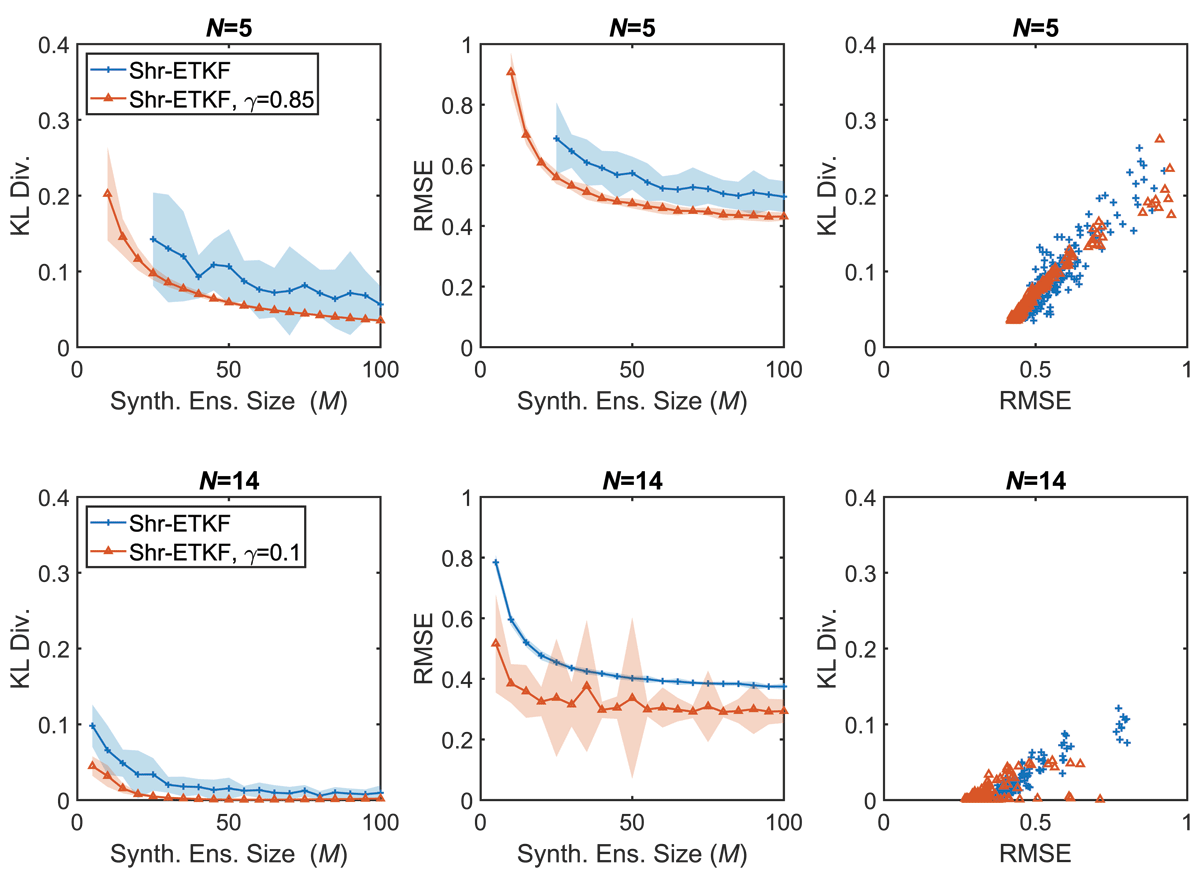
Figure 1
Results for the L96 problem with dynamic ensembles sizes of N = 5 and N = 14, inflation factor α = 1.1, and different synthetic ensemble sizes M. We compute the KL divergence of the rank histogram (4.2) and the RMSE (4.3) for the methods. Error bars show two standard deviations.
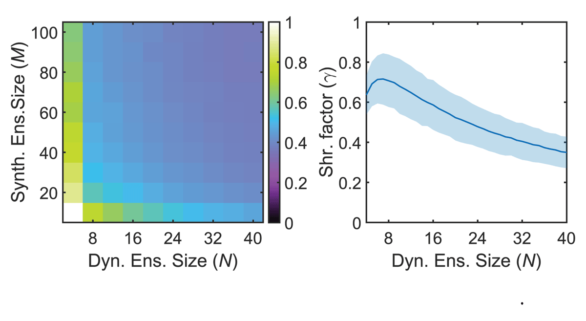
Figure 2
Results for the L96 problem. The left panel presents the analysis RMSE for various values of the dynamic and synthetic ensemble sizes. The right panel presents the shrinkage factor γ (2.15) for a synthetic ensemble size of M = 100 over a number of assimilation steps, with error bars showing two standard deviations.
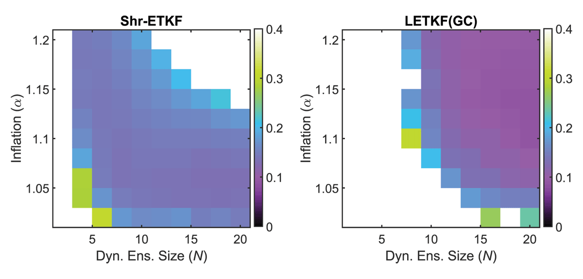
Figure 3
Analysis RMSE results for the QG model. The experiments use a synthetic ensemble size M = 100 and Gaussian samples. Results are compared against LETKF with the Gaspari-Cohn decorrelation function (GC).
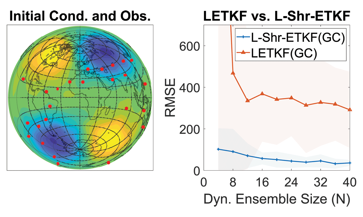
Figure 4
Left panel: initial condition of the water height with blue represented lower than average and yellow representing higher than average, and observation locations (red points). Right panel: analysis RMSE for the localized shrinkage ETKF, and the localized ETKF with the Gaspari-Cohn decorrelation function, with the error bars representing two standard deviations.