
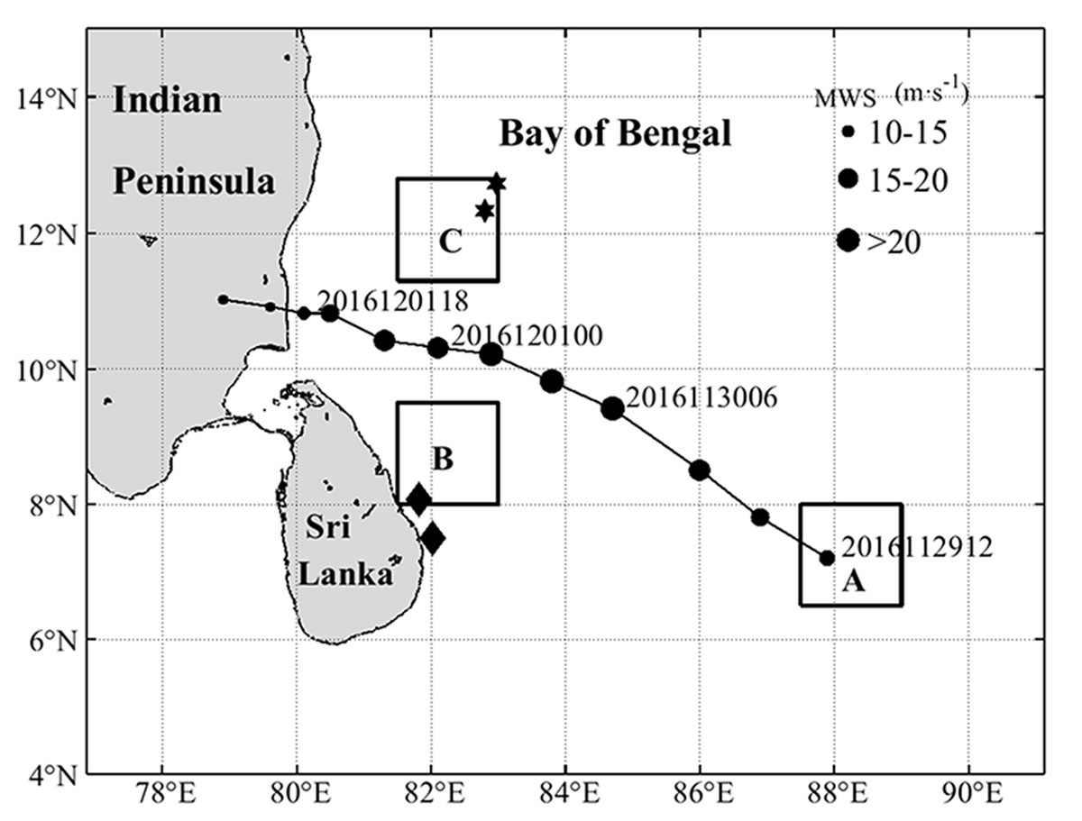
Figure 1
Trajectory of Nada.
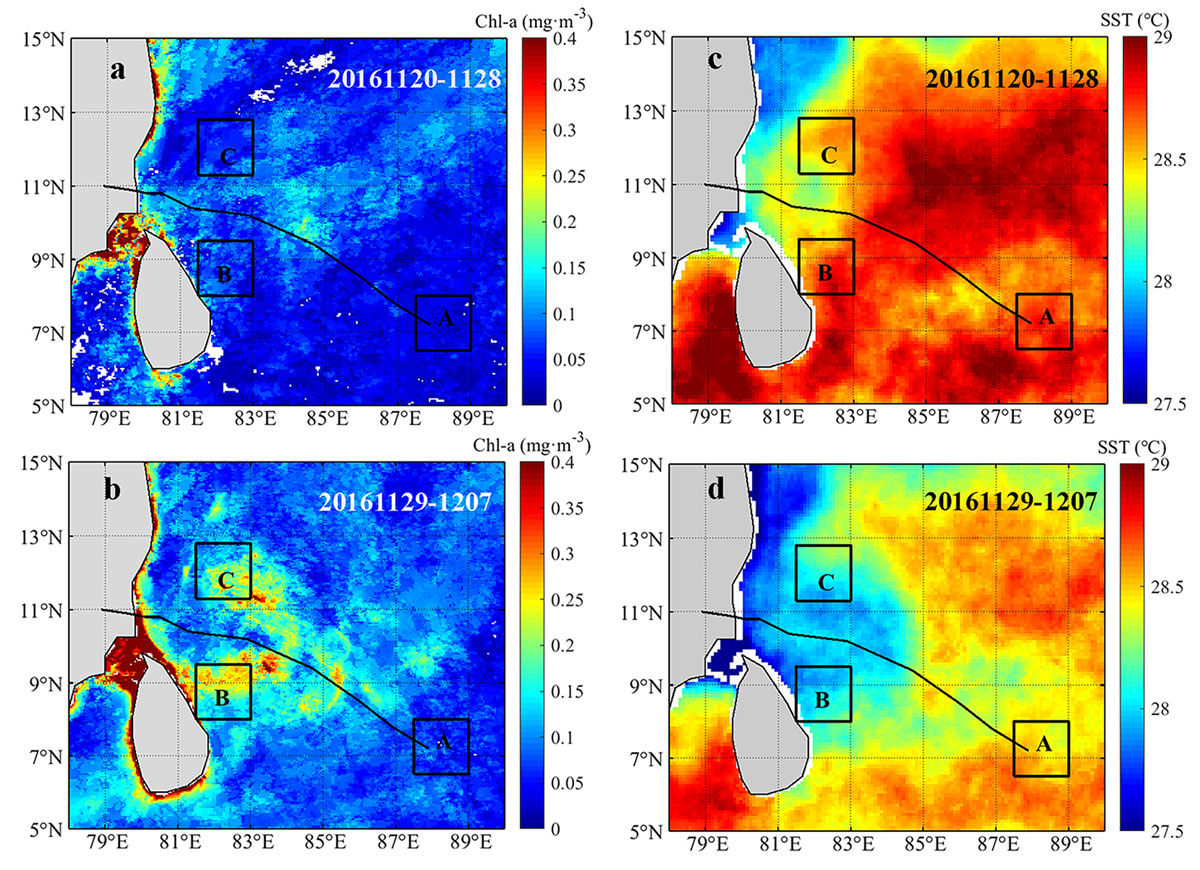
Figure 2
The responses of 9-day averaged surface Chl-a concentration (a, b) and SST (c, d) before (a, c, November 20–28), during and after (b, d, November 29 to December 7) the passage of Nada.
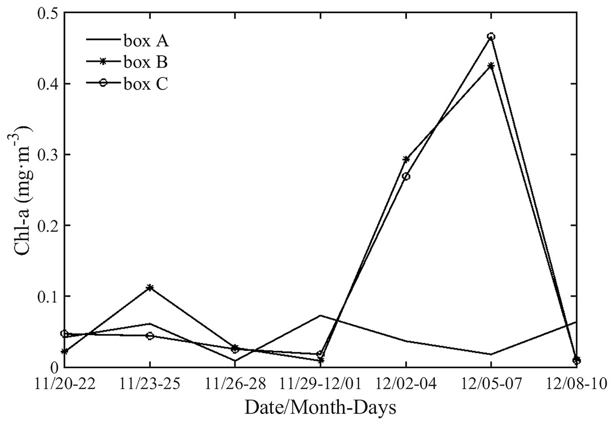
Figure 3
The time series of 3-day averaged Chl-a concentrations in boxes A, B, and C from November 20 to December 10.
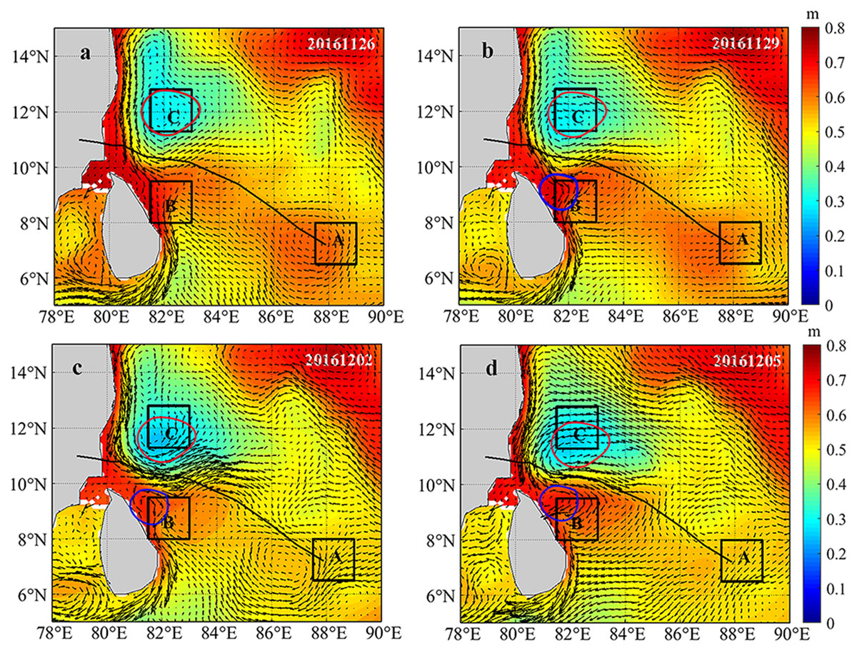
Figure 4
SSH (colors, m) and sea surface current field (arrows, m·s–1) before (a), during (b) and after (c, d) the passage of TC Nada. The red (blue) ring marks the location of the cyclonic (anticyclonic) eddy.
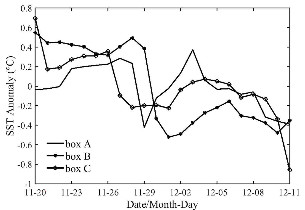
Figure 5
Spatially averaged SST anomaly in boxes A, B, and C from November 20 to December 11.
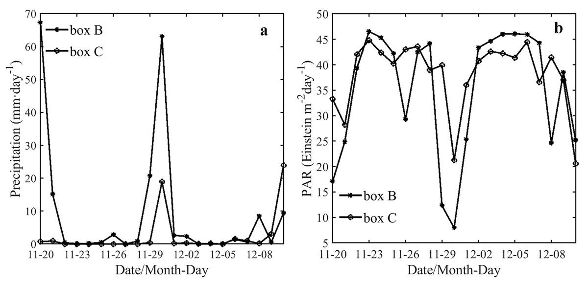
Figure 6
Time series of spatially averaged precipitation (a) and PAR (b) in boxes B and C from November 20 to December 10.
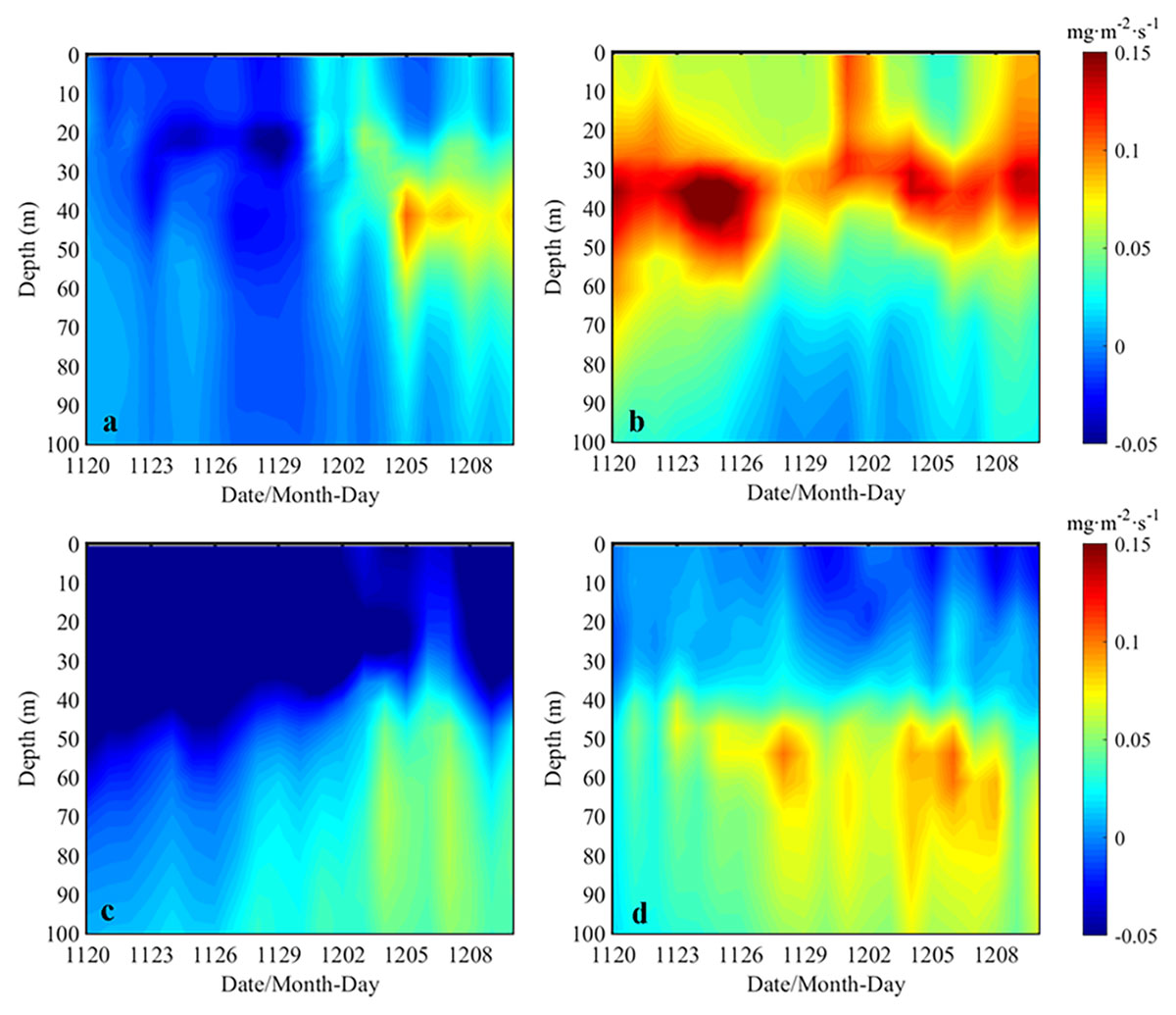
Figure 7
Time series of lateral Chl-a fluxes for box B (east boundary (a), west boundary (b), south boundary (c), and north boundary (d)).
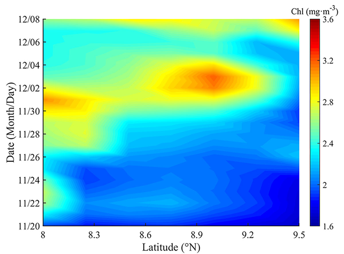
Figure 8
Time series of vertical integration of Chl-a concentration in the upper layer (0–20 m) along the western side of box B from November 20 to December 8.
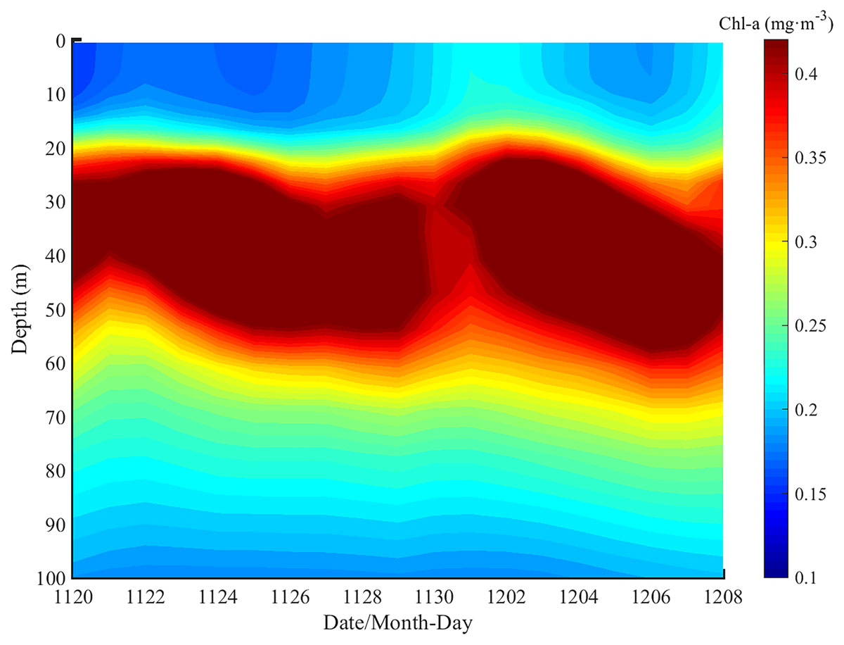
Figure 9
Time series of the domain averaged Chl-a concentration with depth in box B.
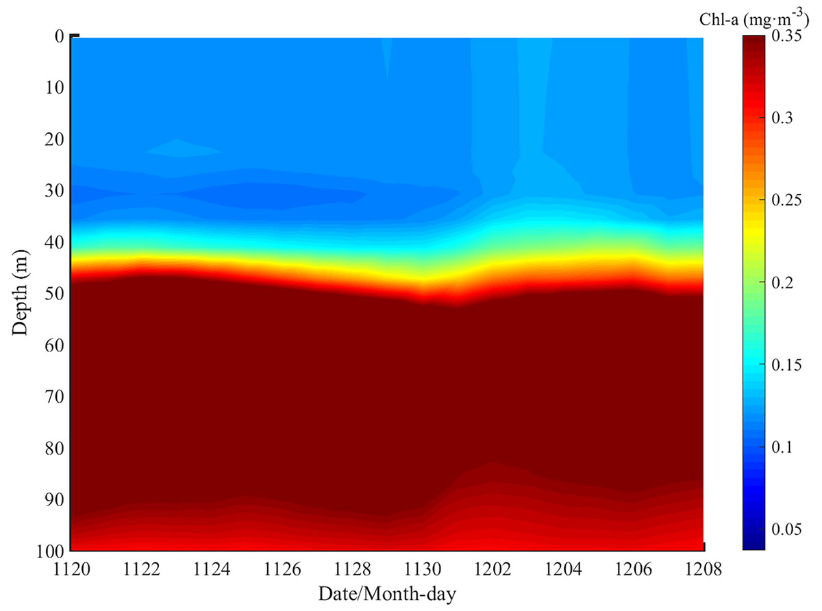
Figure 10
Time series of the averaged Chl-a concentrations with depth in box C.
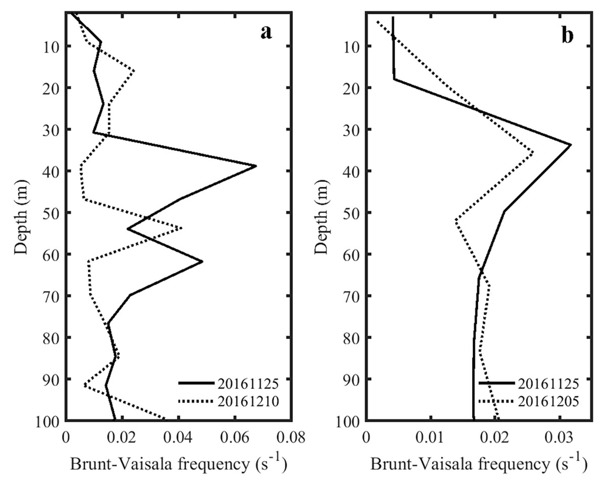
Figure 11
The buoyancy frequency of the Argo profiles in boxes B (a) and C (b) before and after the passage of Nada.
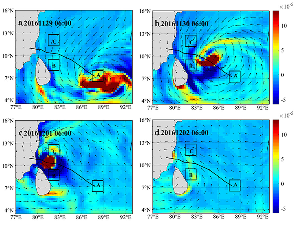
Figure 12
The sea surface wind speed (arrows) and EPV (colors) during TC Nada passage.
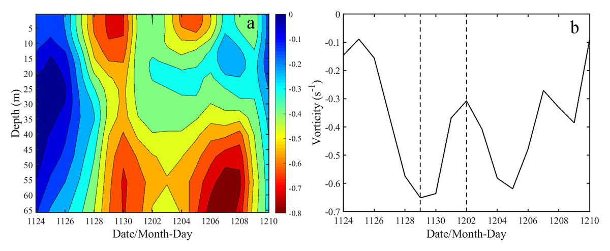
Figure 13
Time series of the averaged vorticity at different depths (a) and at the sea surface (b) of the anticyclonic eddy in box B. Dashed lines present the passage of Nada.
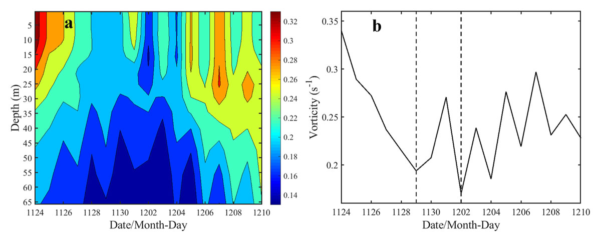
Figure 14
Time series of the averaged vorticity at different depths (a) and at the sea surface (b) of the cyclonic eddy in box C. Dashed lines present the passage of Nada.