Perspective Paper on Lorenz (1982): “Atmospheric Predictability Experiments with a Large Numerical Model”

1. Introduction

How far into the future can weather be predicted? This question has engaged scientists since the advent of numerical weather prediction (NWP). From the simplified model of Lorenz (1963), it became clear that, in a chaotic system, there exists a forecast horizon beyond which little useful information about the future state remains. This behaviour became known as deterministic chaos: a system governed by deterministic equations but highly sensitive to small perturbations. Although the model was not directly applicable to the real atmosphere, subsequent studies examined error growth in what were, at the time, state-of-the-art NWP models (e.g. Charney et al., 1966). Lorenz (1969a) theoretically described the growth of small-scale perturbations into larger scales and estimated the limit of predictability. In Lorenz (1969b), a large set of atmospheric analyses was used to identify atmospheric states that were relatively close to one another (i.e. analogues) and to compare how the differences between them evolved. That study also introduced the average maximum separation of two atmospheric states as an upper bound on forecast error.

In 1981, Edward Lorenz was on sabbatical from MIT at the European Centre for Medium-Range Weather Forecast (ECMWF). ECMWF had begun operational global forecasting in 1979, and Lorenz took the opportunity to investigate predictability in these forecasts. The results were published in Lorenz (1982), which is the focus of this review and is hereafter referred to as L82. L82 approached this question by attempting to estimate upper and lower bounds on forecast error. The upper bound represented what could be achieved by the forecast system at the time, as measured by the skill of a set of forecasts from winter 1980/81; this is what we would now refer to as practical predictability. The lower bound was estimated by comparing two successive forecasts, taking one of them as a proxy for the truth. In modern medium-range forecasting terminology, this is commonly referred to as potential predictability.

Forecast errors in the current forecasting system, which determine practical predictability, arise from both initial-condition errors and imperfections in the forecast model, leading to systematic (bias) and non-systematic errors. Systematic errors may be present almost from the start of the forecast and may also be embedded in the initial conditions because the forecast model is used in the data-assimilation cycle. If such biases grow during the forecast integration, this is often referred to as model drift. Systematic errors may also depend on the prevailing weather regime. Errors of this kind may appear random when verification is aggregated over all situations, but systematic when verification is conditioned on specific regimes. When forecast skill is evaluated against observations, differences in representation between observations (often point measurements) and model output (typically grid-box averages) must also be considered. Representation errors may be systematic (e.g. an anemometer located in an unusually windy position) or random (e.g. precipitation from a local shower). Because this variability occurs within the model grid box, it should be treated as uncertainty rather than as forecast error when observations are compared with model fields (Saetra et al., 2004).

Estimating the lower bound of forecast error can be approached by assuming that the model is perfect and by imposing a lower bound on the initial-condition error. This can be tested in a modelling framework by comparing two model simulations. However, this method relies on the model being able to simulate the intrinsic growth of errors correctly; otherwise, the estimated limit of predictability may be misleading.

L82 was one of the first articles to explore practical predictability in operational forecasts and to propose an approach to potential predictability. This article reviews several key aspects of L82 and relates them to subsequent research. The outline of this paper is as follows. Section 2 reviews the error-growth framework introduced in L82 and its later refinements; Section 3 examines how different mechanisms operating across scales shape error growth from small perturbations to long-range predictability; Section 4 assesses how far the forecast improvements envisaged by Lorenz have been realised in ECMWF forecasts since 1981; Section 5 considers what machine-learning forecasts reveal about the Lorenz framework and its interpretation; Section 6 discusses what L82 implies about the remaining scope for further gains in forecast skill; Section 7 shows how predictability and error growth depend on the variable being forecast; and Section 8 places L82 in a broader context by discussing related developments not addressed directly in the original paper.

2. Error Growth Model from L82 and Further Developments

This section provides a brief review of the development of the parametric error-growth model used in L82. As background, Figure 1a shows the global root-mean-square error (RMSE) of 500 hPa geopotential height (z500) from a recent forecasting system. The forecasts considered here are from the control (unperturbed) members of the ECMWF sub-seasonal forecasting system based on the Integrated Forecast System (IFS) model, run with a horizontal grid spacing of 36 km for the period from 1 April 2025 to 31 March 2026 and covering lead times of up to 45 days. During this period, the ECMWF forecasting system used model version IFS 49r1. The forecasts are verified against the 12-hour-window 4D-Var analysis from the 9 km version of the same IFS model. Although the forecasts were initialised from the 8-hour-window analysis, the two analyses share a substantial part of the analysis error.

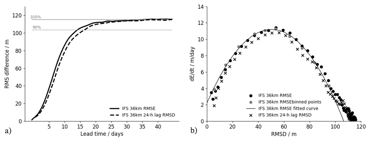
Figure 1

In L82, predictability was assessed by calculating the difference between two forecasts initialised X days apart but valid at the same time, Y days into the older forecast. If X = Y, the latter forecast is at day 0, corresponding to verification against the analysis of that day. This provides a measure of the practical predictability, that is, the forecast skill of the system in 1980/81. By contrast, comparing two forecasts initialised 1 day apart (X = 1 day) provides an estimate of potential predictability, under the assumption of a perfect model and with the initial-condition error taken to be equal to the 24-hour forecast error. In Figure 1a, the RMS curves for X = Y (forecast error) and X = 1 day (hereafter referred to as the 24-hour lagged forecast) are shown; these correspond to the uppermost and lowermost curves in Figure 1 of L82.¹

A key element of L82 was to plot the growth rate of the forecast error (dE/dt) as a function of the error magnitude (E) itself. Figure 1b shows this relationship for the error data in Figure 1a. The method is based on the assumption that, in a chaotic system, the growth rate of the error depends on the magnitude of the error, leading to exponential error growth:

where α is related to the effective Lyapunov exponent of the dynamical system and determines the intrinsic chaotic growth of errors (Boffetta et al., 1998, and references therein). Because the maximum error is constrained by the dynamical range of atmospheric variables and therefore cannot grow without bound, a negative quadratic term was added so that large errors grow more slowly and eventually approach an asymptotic level, as discussed in Lorenz (1969b). On this basis, Lorenz fitted the following function:

The basic model of L82 can be reformulated slightly to better isolate the processes controlling error growth on different time scales. Dalcher and Kalnay (1987), hereafter DK87, used the following formulation:

Here, E is taken to be the standard deviation of the error, that is, the error after bias correction. DK87 introduced a term S, representing a linear error-growth contribution that has its strongest influence when E is small. The addition of such a linear term had already been discussed in the lecture notes from the ECMWF Annual Seminar 1981 by C. Leith, published in Burridge and Källén (1984), and was probably introduced earlier in Leith (1978). By rewriting the quadratic term in Eq. 2, DK87 obtained the parameter E∞ as the asymptotic limit of the error. Based on the decomposition of RMSE (Murphy, 1988), this asymptotic limit E∞ is given by:

where F was the forecast value valid at the verification time, A is the analysis, and C is the climatological value of the verified variable. The overbar denotes an average over many grid points and forecast cases. In the case of lagged-forecast differences, the variances of the two forecasts may be assumed to be equal.

Integrating the DK87 equation shows that the bias-corrected forecast error as a function of lead time is determined by the initial error (E₀), the intrinsic chaotic error growth of the system (α), the random model error term (S), and the variability of both the atmosphere and the model, which together determine E∞.

One interpretation of S is that it represents the growth of errors in the absence of initial-condition errors, arising from model imperfections. In the case of lagged-forecast differences, both forecasts are produced with the same model, and S should therefore be zero, which appears to be a reasonable assumption from inspection of Figure 1b. However, the interpretation of S as a pure model-error term is debatable. Zhang et al. (2019) and Sun and Zhang (2020), for example, interpreted S as representing rapid error growth associated with convective-scale processes (see discussion in Section 3).

Magnusson and Källén (2013) used the DK87 equation to examine improvements in ECMWF forecast skill from 1986 to 2011, with the aim of separating the effects of reduced initial-condition error and reduced model error by analysing the evolution of the individual terms in Eq. 3. The study concluded that, in particular, the introduction of 4D-Var data assimilation (Rabier et al., 2000) in 1997, together with the subsequent improved use of satellite observations, contributed substantially to forecast improvement by reducing the initial-condition error and, consequently, the error growth associated with α.

One source of uncertainty when applying Eq. 3 to estimate the contributing terms is the calculation of the time derivative dE/dt. To address this difficulty, Žagar et al. (2017) introduced a curve-fitting approach applied directly to the error itself, rather than to dE/dt, while retaining parameters that can still be related to the terms in Eq. 3.

3. Error Growth from Small Errors to Long-Range Predictability: Implications for the Shape of the Parabola

Although the first data point in the L82 version of the figure (Figure 2 in L82) was still relatively far from E = 0, the points nevertheless resembled a parabola. In Figure 1b of the present paper, a second-order polynomial has been fitted to the data following the approach of L82, after first binning the points. The binned values are shown in Figure 1b as grey dots. Here, 10 equally sized bins were used, but only RMSE values below 100 m were included in the fit in order to avoid the influence of long-range forecasts (see below). The current data follow the parabolic form reasonably well, although some deviations are evident for very small and very large errors.

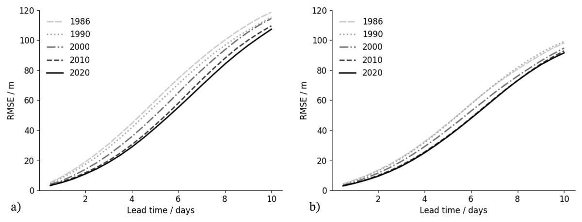
Figure 2

Turning first to the growth of small errors, L82 states in the introduction:

A central point in this quotation is that the atmosphere contains processes with intrinsically rapid error growth on small spatial scales, and that these errors can project onto larger scales through upscale transfer (Lorenz, 1969a). The mechanism of upscale error growth from convective to synoptic scales has been, and remains, an area of active research. Zhang et al. (2007) proposed a three-stage framework consisting of rapid error growth associated with moist convective instability, a transition in which unbalanced perturbations adjust towards balanced structures through geostrophic adjustment, and subsequent growth through baroclinic instability. A similar conceptual model was diagnosed by Baumgart et al. (2018).

Several studies using the L82-style dE/dt versus E diagnostic reported apparently “super-exponential” growth for the smallest errors (e.g. Nicolis, Vannitsem, & Royer, 1995), consistent with the idea of rapid convective- or mesoscale error growth. However, what appears to be very rapid initial growth may also arise from the changing relationship between analysis errors and forecast errors: at short lead times, forecast errors are partially correlated with the analysis error, and as that correlation decays the apparent growth rate is inflated (Simmons & Hollingsworth, 2002). In Figure 1b, this effect is most evident for the first cross in the RMSE data; beyond that point, there is no clear evidence of sustained super-exponential behaviour.

At the other end of the parabola, Lorenz acknowledged already in the introduction that “We shall not be concerned with climatic or other long-range predictability, which should exist if certain features of the atmosphere can still be predicted when most of the atmosphere cannot”. Since L82, extensive research has examined forms of predictability that do not arise primarily from rapid, internally generated growth of small errors, but instead from relatively slowly varying components of the Earth system that act as boundary conditions or external forcings for the mid-latitude atmosphere (e.g. Stan et al., 2017). Examples include tropical forcing associated with slow variations in tropical heating from organised convection (e.g Hoskins & Karoly, 1981) such as Madden-Julian Oscillation (MJO)-related variability, lower-boundary influences from sea-surface temperature, terrestrial influences from soil moisture, snow and sea-ice, and upper-boundary influences from the stratosphere, such as the Quasi-Biennial Oscillation (QBO) and variations in the polar vortex.

Within the framework of the L82/DK87 error-growth model, these slowly varying influences may be interpreted as “slow modes” with weaker intrinsic growth and a longer time to approach saturation (Palmer, 1993; Peña & Kalnay, 2004). When rapid, chaotic atmospheric error growth is combined with slow, externally forced variability, the total error need not approach its asymptotic level at a single rate. Instead, rapid initial growth may be followed by a more gradual increase as the remaining predictable signal becomes increasingly tied to slowly evolving boundary or forcing anomalies. This mixed behaviour is consistent with the tendency in Figure 1b for the largest-error points to lie to the right of the fitted parabola.

Departures from a perfect parabola in the dE/dt versus E plot can therefore reflect the superposition of several growth mechanisms with different characteristic time scales. For very small errors, convective or mesoscale processes, and/or the rapid decorrelation of forecast and analysis errors, can produce an initially steep slope, making the left-hand side of the curve appear too high relative to a simple quadratic fit. At larger errors, the remaining predictable component of the flow may be increasingly influenced by slowly varying, externally forced components, implying weaker effective growth and hence a slower approach to saturation. The resulting curve may therefore be skewed rather than symmetric. Stroe and Royer (1993) examined a more general functional form for the growth law, later revised by Simmons et al. (1995), in which the dependence on normalised error (E/E∞) is not constrained to be linear, as in DK87. They found that the effective exponent varies with season and is often lower than 1, consistent with a slower-than-quadratic reduction in growth as saturation is approached. This skewness has practical implications when diagnosing the different components in Eq. 3, because parameter estimates will depend on whether the fitted data primarily sample the left- or right-hand side of the curve.

4. How Has the Skill of ECMWF Forecasts Evolved Since 1981?

In L82, the potential for forecast improvement was summarised as follows:

It is not entirely clear how Lorenz derived the statement that “ten-day forecasts as good as present seven-day forecasts”. One possible interpretation is that it was based on (1) correcting the forecast mean state and variability over the Northern Hemisphere (20°N–90°N), and (2) assuming that forecast skill over the Southern Hemisphere (20°S–90°S) could eventually match that over the Northern Hemisphere. Alternatively, the statement may have been based on comparing the actual forecast error with the difference between two successive forecasts initialised 1 day apart, as shown in Figure 1 of L82. The latter interpretation would assume that the forecast model can become a perfect representation of the atmosphere, so that the remaining errors arise entirely from the initial conditions. However, if this were the intended method, the implication would be closer to a ten-day forecast performing as well as a present-day 6-day forecast, based on Figure 1 of L82.

Since the start of operational forecasting in 1979, the skill of ECMWF forecasts has improved substantially. Figure 2 shows the RMSE of z500 over the Northern Hemisphere for five snapshot years (1986, 1990, 2000, 2010, and 2020). The figure updates Figure 1 of Magnusson and Källén (2013) by including 1986 and 2020; ECMWF does not retain regular-archive forecasts prior to 1986. The forecasts are verified against the 5th generation of ECMWF Reanalysis (ERA5; Hersbach et al., 2020).

With regard to the statement in L82 about reducing the 1-day error, the 1-day RMSE in ECMWF operational forecasts over the Northern Hemisphere decreased from 19.8 m in 1986 to 5.0 m in 2020, while over the Southern Hemisphere it decreased from 36.9 m to 5.8 m. Thus, since 1986, the error has been halved twice in the Northern Hemisphere and reduced to approximately one-sixth in the Southern Hemisphere; the reduction is even larger if the comparison is extended back to 1981, as documented in Simmons et al. (1995). In the operational ECMWF forecasts, the day-6 error in 2020 is comparable to the day-3 error in 1990 (Figure 2a). These improvements in 1-day forecasts reflect a combination of increased observational coverage, especially from satellites, improved data assimilation that makes better use of the observations, and improved forecast models that provide a more accurate first guess for the assimilation system (Bauer, Thorpe, & Brunet, 2015).

To isolate the impact of the observing system, one can instead examine forecast improvement based on forecasts from ERA5 reanalysis which uses the same forecast model and data-assimilation system throughout the full period but with an evolving observing network (Figure 2b). In this case, the 1-day error decreases from 7.0 m to 4.7 m over the Northern Hemisphere and from 9.0 m to 5.2 m over the Southern Hemisphere. The lower errors for the ERA5 forecasts than for the operational ECMWF forecasts in 2020 are partly due to the ERA5 analysis using a longer 12-hour assimilation window, which incorporates observations 4 hours later into the forecast, and partly because ERA5 analyses are also used for verification, which favours the ERA5 forecasts.

5. Lorenz Error Growth Model in the Light of Machine-Learning-Based Forecasts

The emergence of machine-learning weather prediction (MLWP; Bi et al., 2023; Lam et al., 2023; Lang et al., 2024) has brought renewed attention to several of the issues discussed in L82. Figure 3 shows the RMSE and the RMS difference for lagged forecasts from the 9 km version of the physics-based IFS model (the same version as discussed in the previous sections) and from the deterministic ECMWF Artificial Intelligence Forecasting System (AIFS-single), with a horizontal resolution of approximately 25 km (Lang et al., 2024; Moldovan et al., 2026). The AIFS-single are initialised from the same initial conditions as the IFS forecasts. Verification is based on the same region and period as in Figure 1.

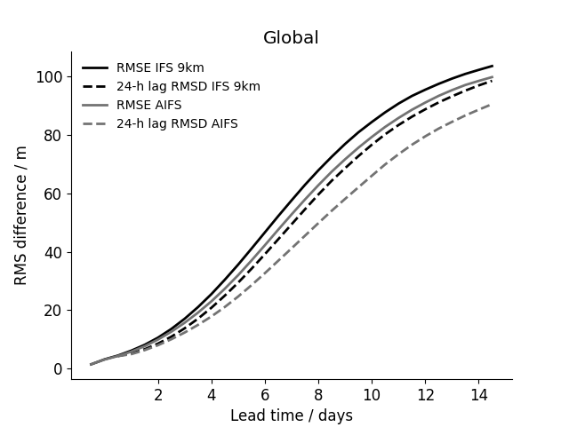
Figure 3

AIFS-single exhibits slower error growth than the IFS forecasts. This immediately raises the question of which components of the error-growth model account for the difference. Because both forecast systems are initialised from the same IFS analysis, differences in the initial-condition error (E₀) can be excluded.

A central issue in the discussion of first-generation ML-based forecasting systems has been the role of smoothing. This is not a new concern: in Section 4, L82 discusses the implications of differences in mean state and variance between the forecast fields and the verifying analysis. Lorenz states:

If a forecast is smoother than the truth, the RMSE can be reduced by avoiding the double-penalty effect, whereby spatially displaced but otherwise realistic structures are penalised twice. In the limiting case in which all skill is lost and forecasts and analyses are uncorrelated, a forecast with the correct variance has an RMSE that is $\sqrt{2}$ times larger than that of a forecast equal to climatology, as follows from Eq. 4. For example, smoothing is obtained in an ensemble-mean forecast, as the ensemble mean approaches climatology then the ensemble members become mutually uncorrelated (Bengtsson, Magnusson, & Källén, 2008).

In NWP, excessive numerical diffusion historically produced forecast fields that were too smooth. Over the past decade, however, forecast variability for upper-air variables such as z500 has become very close to that of the verifying analysis. The issue of smoothness has re-emerged with the advent of MLWP. Because these systems are currently trained to minimise the (R)MSE at specific lead times (e.g. 72 hours in the case of AIFS; Lang et al., 2024), the training procedure can favour different degrees of smoothing. In AIFS, the smoothing appears to be largely confined to sub-synoptic scales (wavenumbers greater than 20), which are less predictable (e.g. McTaggart-Cowan et al., 2026). This loss of forecast variability increases somewhat with lead time, so that AIFS acts, in effect, somewhat as a filter on the unpredictable scales. However, the relative reduction in the asymptotic error is much smaller than for an ensemble-mean forecast (not shown) and is probably insufficient to explain the full difference between IFS and AIFS.

One might also expect ML-based forecasts to reduce both systematic and random model errors. For several variables and regions, this is indeed the case. For z500 outside the tropics, however, the RMSE is dominated by the random component of the error. Applying a bias correction before calculating the RMSE for z500 produces only a small change (not shown).

A reduction in random model error in AIFS would act to reduce the term S in Eq. 3. However, if one considers the lagged-forecast difference, which contains no contribution from model error, the contrast between IFS and AIFS-single is even larger for the lagged-forecast curves (Figure 3, dashed lines). We can therefore conclude that the difference is (at least partly) associated with the intrinsic chaotic error growth (α) and/or with the forecast-variability term ((F–C) in Eq. 3), which influences the asymptotic limit (E∞), without excluding some contribution from S as well.

6. So How Much Further Can the Forecasts Be Improved?

In L82 it was stated, “A study by Lorenz (1969a) indicated that even if the larger scales could be observed perfectly, the inevitable uncertainties in the smaller scales would after a day or so induce errors in the larger scales…”. This would put a limit on the predictability of the atmosphere. One way to explore this limit is to evaluate the divergence of two forecasts during model integration. In L82, this was done in a simple way by comparing consecutive operational forecasts. In 1980, forecasts were produced once per day, hence the 24-hour separation between initial times. In Figure 4, we compare the result from L82 with recent forecasts for the period 1 December 2023 to 10 March 2024 based on the 36-km ECMWF forecasts. The RMSE for the 9-km version, available out to 15 days, is also included, together with the RMS difference from the “accidental twin” experiment (see below). Finally, the figure includes the average RMSE of the 36-km forecast over days 40–45 as a measure of the asymptotic limit, together with 90% of that value.

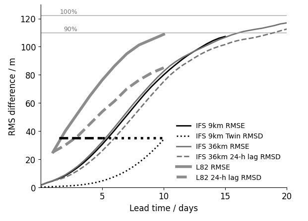
Figure 4

Comparing the RMSE and the lagged-forecast difference shows that the two curves for the recent period are much closer together than in L82, indicating that the current forecasting system is much closer to the “perfect-model”. However, the lagged-forecast curve in L82 was not a good estimate of the upper limit of predictability because smoothing reduced the asymptotic level of the lagged-forecast difference.

An alternative approach to explore the potential predictability is to add perturbations to the initial conditions and rerun the forecast with the same model to examine how the difference between the two “twins” grows. This provides an opportunity to test different perturbation amplitudes, corresponding to different assumptions about the quality of future initial conditions. The method has the caveat that the perturbations must be constructed so that their growth is representative of the expected forecast-error growth. Twin experiments also assume a perfect model, that is, zero model error, and require that the model realistically simulates the intrinsic growth of errors. While this is generally believed to be a reasonable assumption on synoptic scales in the mid-latitudes, it has been more questionable at convective scales, as already noted in L82.

In recent years, several studies have attempted to estimate the limit of predictability using model twin experiments (e.g. Judt, 2018; Selz, 2019; Zhang et al., 2019). These studies used kilometre-scale global models, which are thought to capture error growth on convective scales more realistically, as discussed above. They all applied perturbations of very small amplitude, typically 1–10% of the current analysis error. Zhang et al. (2019), however, found little sensitivity of synoptic-scale error growth to explicitly resolving convection. That study concluded that the then-current predictability limit could be extended by about 5 days if initial-condition errors were reduced to extremely low levels.

At ECMWF, two almost identical operational forecasts were run from late June 2023 to November 2024 using a 9-km model grid spacing. Although the two forecasts had identical initial conditions and model formulation, the surface orography differed by less than one metre, and some other static surface specifications also differed slightly, so the runs were not bit-identical. This “accidental twin experiment” therefore provided a pair of forecasts whose differences grew from minimal perturbations. The RMS difference between the two forecasts is included in Figure 4.

The results in Figure 4 show that the current 5-day forecast error (35 m) is similar to the 1.5-day error in 1980/81, implying an improvement of about 3.5 days over the past 44 years. In the accidental twin experiment, the same level of difference is reached at around day 10, as marked by the black dashed and dotted lines in Figure 4. For this dataset, 90% of the 25–30 day error level is reached just after day 15 for the 36-km version of the current model (the final point of the 15-day forecast for the 9-km version lies just below the 90% line). If the accidental twin experiment were to continue growing beyond day 10 in a similar manner to the lagged forecast difference from the operational forecast, this would suggest an upper bound on predictability of approximately 20–22 days for the metric used here. However, the choice of threshold, here 90%, for defining the point at which no useful skill remains introduces an unavoidable degree of arbitrariness into estimates of the predictability limit.

7. Fitting the Lorenz Model to Other Parameters

In the conclusion of L82, it is also stated:

To illustrate this point, Figure 5 shows the RMSE over Europe for both z500 and 10-metre wind speed, verified against observations (SYNOP for wind and radiosondes for z500) and averaged over the period 1 April 2025 to 31 March 2026. It is immediately apparent that the 12-hour forecast error (the first point) for wind speed is much larger, relative to the asymptotic limit, than for z500. This is partly related to sub-grid-scale variability (representativeness error), which is captured by the observations but not by the model output, as well as to rapidly developing model biases (see the discussion of different error types in the Introduction section). Another possible contributor is larger analysis error in near-surface winds. Nevertheless, during the forecast the loss of the remaining predictability is broadly similar to that seen for z500, as anticipated in L82. The maximum error growth, however, appears to occur at somewhat shorter lead times for 10-metre wind speed than for z500. One possible explanation is that different variables are most active on different horizontal scales and therefore exhibit different characteristic time scales of error growth, since predictability is lost more rapidly on shorter time scales (Lorenz, 1969a; Žagar et al., 2017).

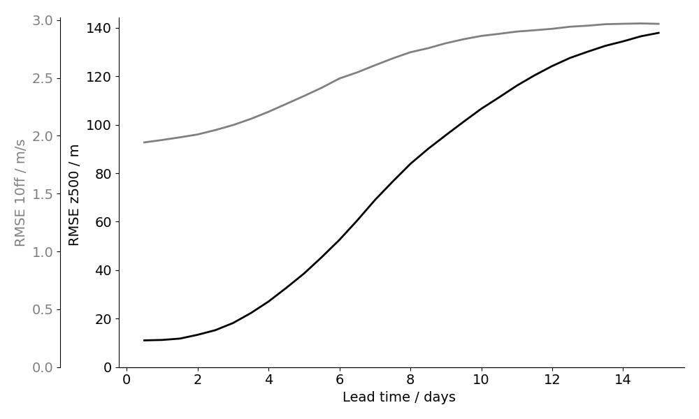
Figure 5

In the medium range, variability in the mid-latitudes is dominated by Rossby-wave dynamics, which strongly imprint on z500. In the tropics, variability is more complex: strong convection in the ITCZ can produce rapid error growth, while the large-scale flow is also modulated by much slower modes such as the MJO and ENSO. The implications for predictability were explored by Judt (2020). On synoptic scales, tropical variability is also influenced by atmospheric tropical wave modes. Žagar et al. (2017) applied the L82 framework for different types of tropical waves using a normal-mode basis that takes both wind and geopotential into account. Using the ensemble spread as a proxy for the forecast error, they found that unbalanced (gravity-wave) modes exhibited a faster loss of predictability than balanced modes such as equatorial Rossby waves.

8. Discussion

The landmark paper by Lorenz (1982) provided one of the first published assessments of global forecast skill from an operational NWP model and, at the same time, introduced a conceptual framework for understanding forecast errors and their possible reduction.

L82 examined forecast skill averaged over 100 days during boreal winter. While long-term improvements in forecast systems are important to document, it is also reasonable to ask how relevant an average predictability limit is in practice. Although the RMSE for a season or a year provides a measure of mean forecast performance, forecast skill fluctuates substantially from day to day. Occasional episodes of particularly rapid error growth are commonly referred to as forecast busts or drop-outs. The error growth associated with such events has been the subject of extensive research (e.g. Grams, Magnusson, & Madonna, 2018; Hauser et al., 2026; Magnusson, 2017; Rodwell et al., 2013).

One way to address the day-to-day variability of forecast skill is to run an ensemble forecast system in order to estimate the evolving forecast uncertainty. To obtain a reliable estimate of that uncertainty, however, all major sources of forecast error must be represented (Rodwell et al., 2016). Here too, the L82 framework remains informative, as explored by Bengtsson, Magnusson, & Källén (2008). In this context, an ensemble system must simulate realistic initial-condition errors (Magnusson, Nycander, & Källén, 2009), include a representation of non-systematic model error (Leutbecher et al., 2017), and employ a model formulation that yields realistic intrinsic error growth and asymptotic error limits (Bengtsson et al., 2008). In the past, it was often difficult to obtain sufficient ensemble spread relative to the ensemble-mean error. In many cases, this was due to insufficient variability in the forecast model, which led to too low an asymptotic limit of the ensemble spread. This behaviour is captured much better today, at least for upper-air variables such as z500 (see, for example, Figure 9 in Haiden et al., 2025). For surface variables, however, sub-grid variability, observation errors, and systematic forecast errors must be taken into account before ensemble spread can be meaningfully compared with ensemble-mean error (Saetra et al., 2004). Understanding the different components of forecast error is therefore essential when evaluating an ensemble prediction system.

Coming back to the first question of “How far into the future can weather be predicted? and following “how can the forecasting system be improved to narrow the gap between practical and potential predictability?”, the accidental twin experiment presented here may serve as an upper estimate of predictability. However, it assumes that it realistically captures the intrinsic growth of errors, but probably more importantly, it is also not realistic to expect that such minimal initial-condition errors can be achieved in practice. This is partly due to limitations in observational coverage and to observation errors that constrain mesoscale data assimilation (Majumdar et al., 2021). Moreover, the rapid growth of convective-scale errors and their upscale transfer raise the question of whether reducing initial errors on convective scales will be worth the required effort. On the other hand, the results for 10-metre wind error suggest that, for near-surface variables, there remains considerable room for improvement before this limit is approached. Whether this is most effectively achieved through model development, post-processing, or ML-based forecasting remains to be seen. While efforts to reduce these errors continue, the associated uncertainties must also be estimated and communicated appropriately.

Recent results from MLWP have begun to challenge current estimates of error growth and to suggest a substantially longer potential predictability horizon (Vonich & Hakim, 2025). With regard to chaotic error growth, Selz and Craig (2023), followed by Selz and Craig (2025), discussed slower difference growth on small, convective scales in MLWP models. However, the results presented here also indicate reduced growth at larger error magnitudes. This raises several questions: (1) What is the relationship between lead-time-dependent smoothing at specific scales, which affects E∞, and the intrinsic chaotic error growth parameter α? (2) Does smoothing at convective scales reduce α for synoptic scales? (3) How does α diagnosed from the difference between two forecasts (e.g lagged forecast), relate to α diagnosed from the difference between a forecast and the truth (i.e forecast error)?

Answering these questions will require further research. In particular, addressing the first question may require extending the growth model to individual wavenumbers, or to spectral bands, while allowing E∞ to depend explicitly on lead time. The second question leads back to the problem of scale interactions and upscale error growth discussed already by Lorenz (1969a) and more recently by Rotunno and Snyder (2008) and Sun and Zhang (2020). One possible hypothesis is that smoothing a strong but intrinsically unpredictable convective outflow could reduce errors in the Rossby-wave forcing, following the mechanism described by Zhang et al. (2007), and thereby reduce downstream error growth along the Rossby-wave guide. This idea, however, remains to be tested. Addressing the third question may require genuinely new developments in the study of forecast-error growth.

Taken together, these considerations show that forecast-error growth and the limit of atmospheric predictability remain active and important areas of research, nearly half a century after Edward Lorenz’s seminal study in Tellus.