
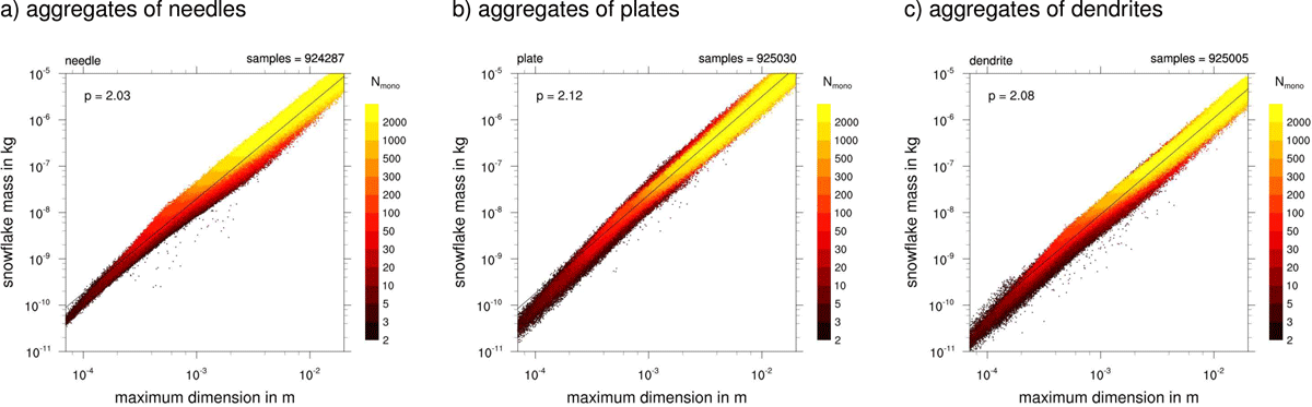
Figure 1
Scatter plots showing the mass-size relations for aggregates of needles, plates, and dendrites. Colors indicate monomer number N, and the regression line represents the power-law fit with fractal exponent p for .
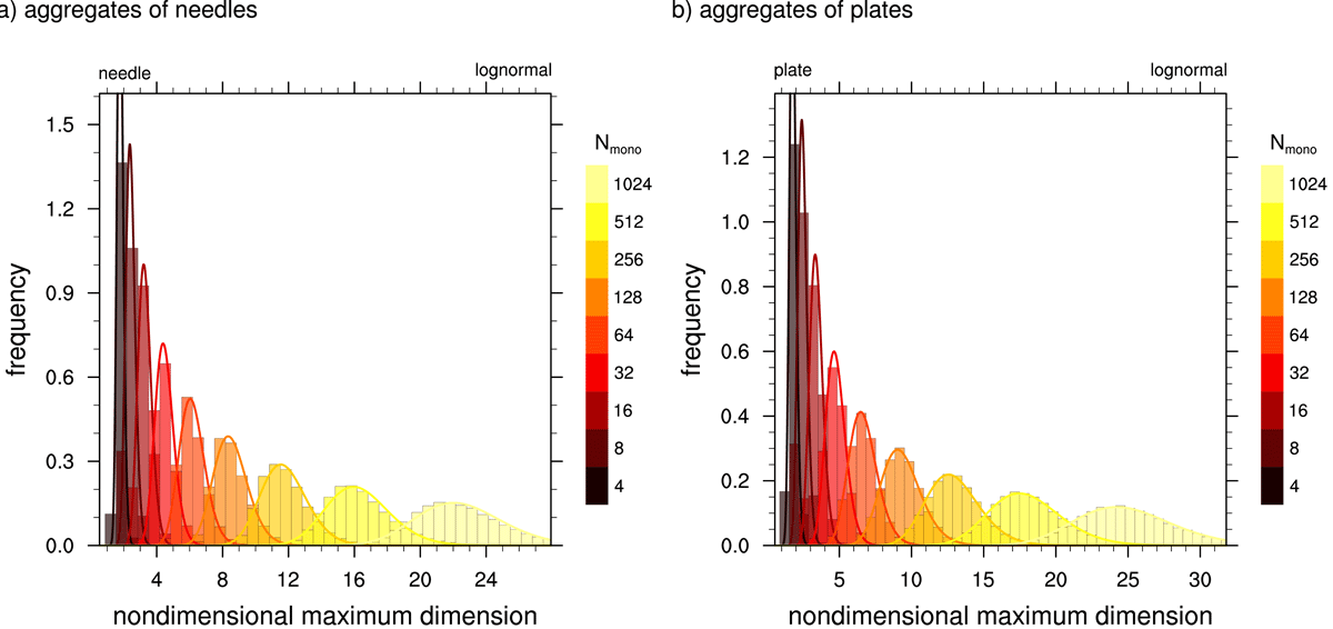
Figure 2
Histograms of the nondimensional maximum dimension for aggregates of (a) needles and (b) plates for different monomer numbers N. Solid lines show lognormal distributions with the same mean and standard deviation as the corresponding datasets. Results for dendrite aggregates are similar and are omitted for clarity.
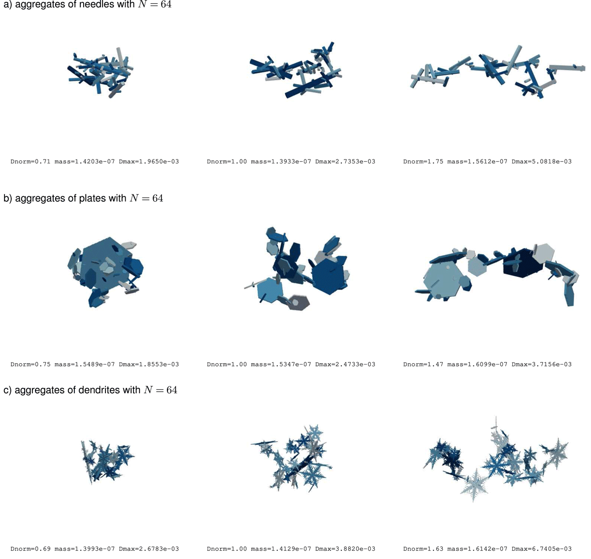
Figure 3
Examples of aggregates of needles, aggregates of plates, and aggregates of dendrites for monomer number and different . For each aggregate, the normalized diameter , the mass m in kg, and the maximum dimension in m are given. The snowflakes with (left column) are much smaller in terms of maximum dimension than the elongated snowflakes with (right column). The central column shows an example of the mean aggregate snowflake with for the given N. The aggregate mass m in each row is similar, but not identical. The color shading does not have a physical meaning and is used solely to help distinguish individual monomers within the aggregates.
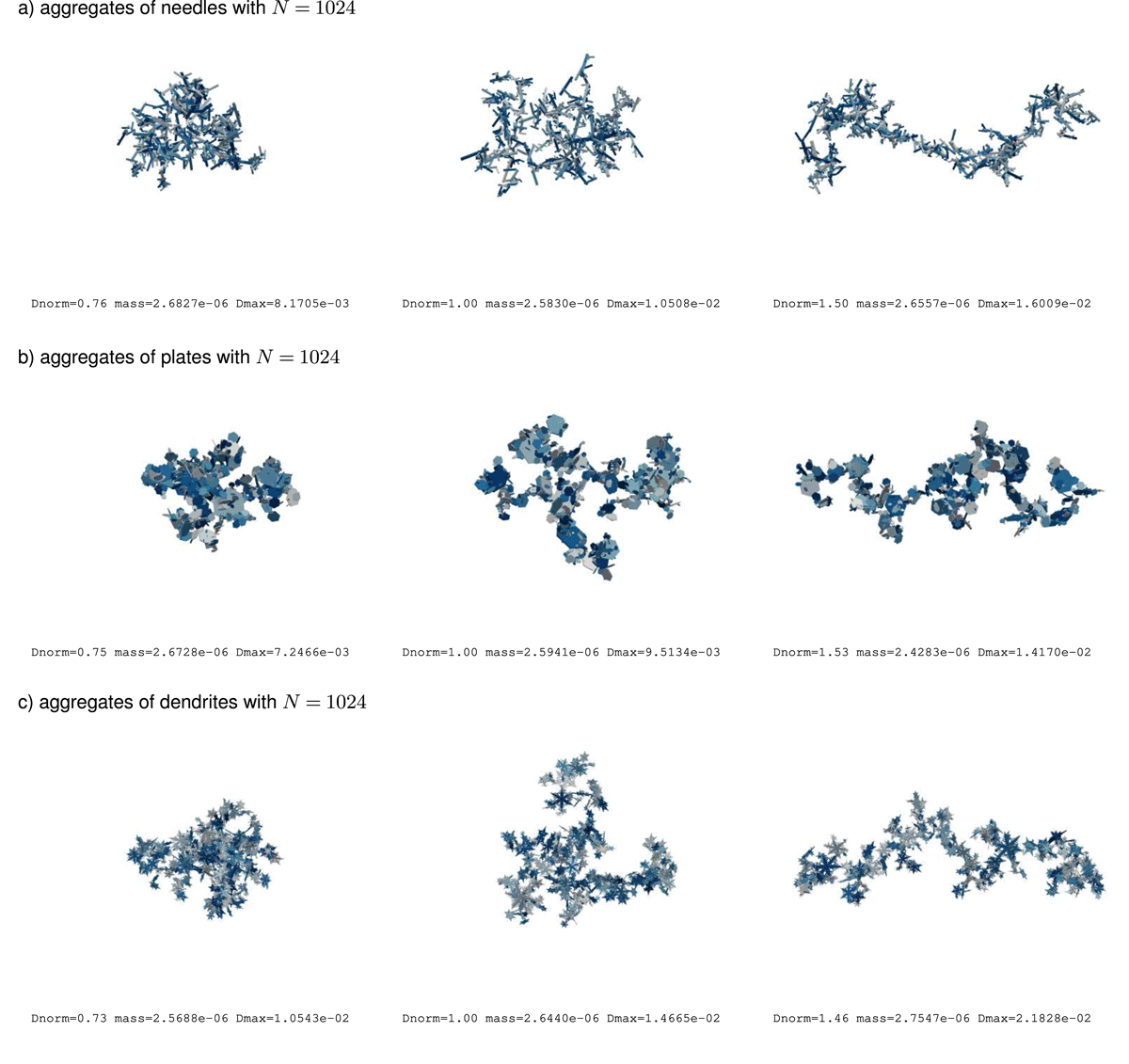
Figure 4
As Figure 3, but for a monomer number of .
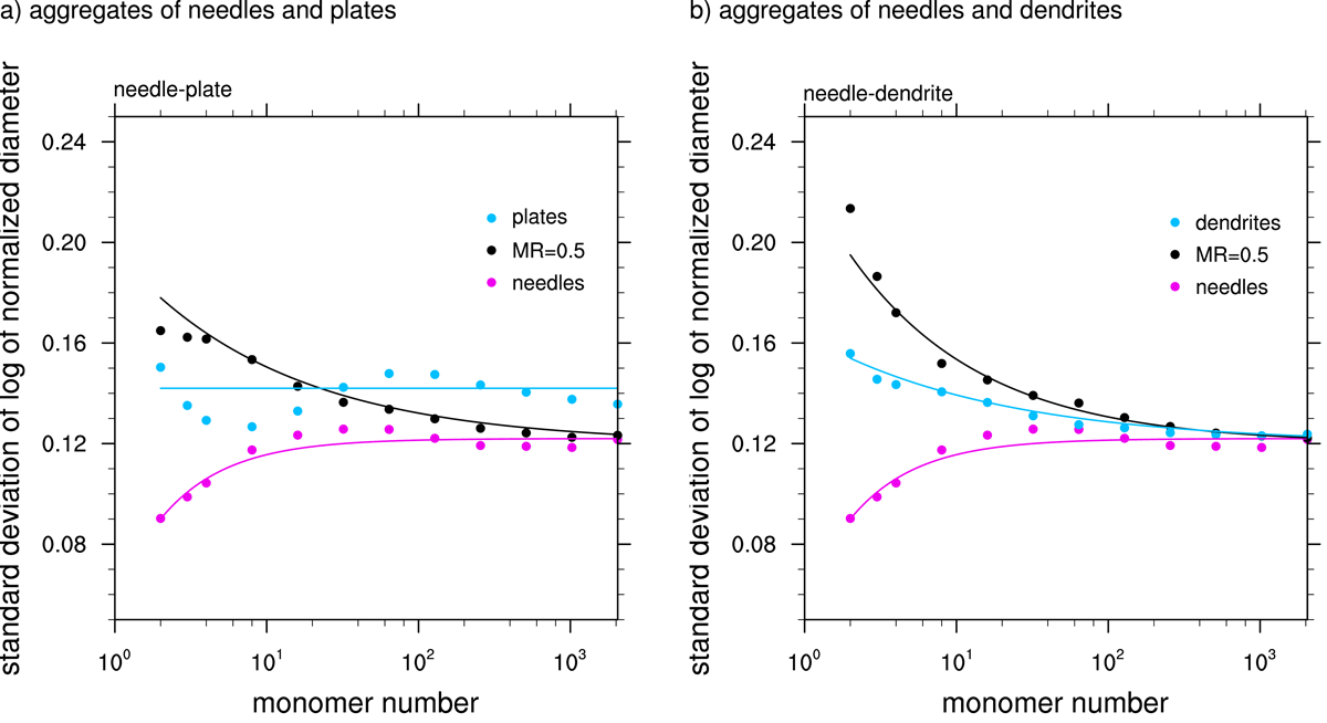
Figure 5
Standard deviation of the normalized diameter as a function of monomer number N for aggregates of plates, aggregates of needles, and mixture aggregates of plates and needles (left), and aggregates of needles, aggregates of dendrites, and mixture aggregates of both (right). Aggregates of mixtures are shown for different monomer ratios MR. The solid lines are the parameterizations using Eqs. (6)–(10).
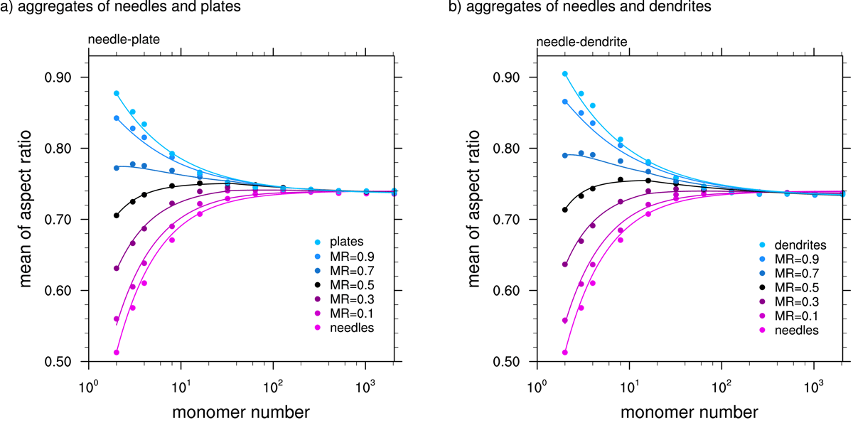
Figure 6
Mean horizontal aspect ratio of aggregates of needles and plates (left) and aggregates of needles and dendrites (right) as a function of monomer number N. Aggregates of mixtures are shown for different monomer ratios MR. Note that the data for pure needle aggregates is the same in both plots. The solid lines are parameterizations using Eqs. (11)–(15), with intermediate values linearly interpolated between (needles), (plates or dendrites), and .
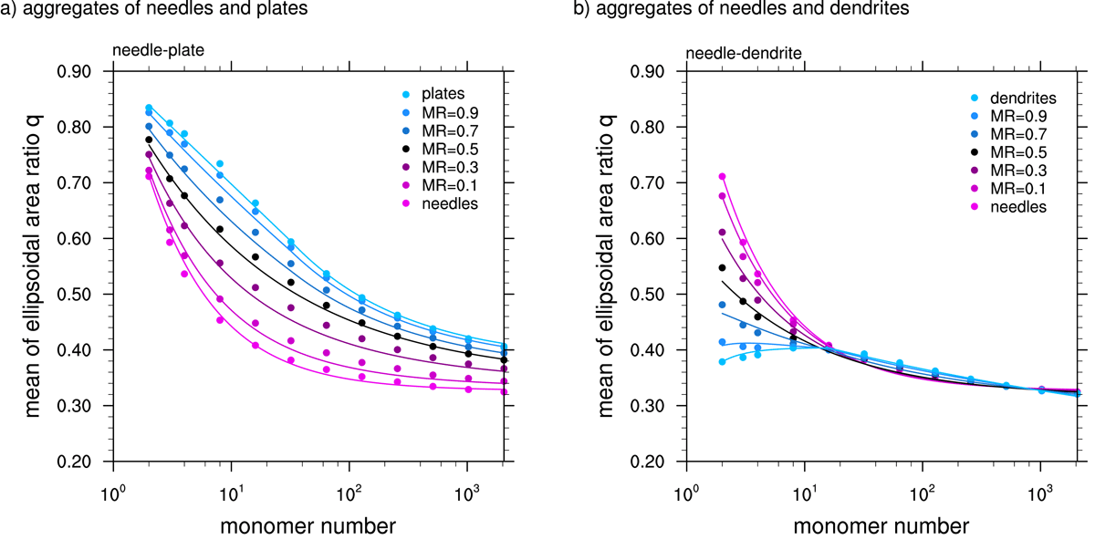
Figure 7
As Figure 6 but for the mean ellipsoidal area ratio q. The solid lines are the parameterizations using Eqs. (16)–(20).
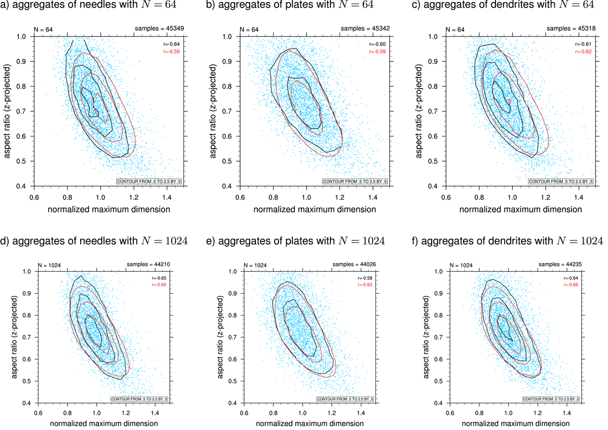
Figure 8
Joint PDF of the normalized maximum dimension and the aspect ratio for different monomer habits and monomer numbers. The blue dots show thinned-out samples of the dataset, black isolines correspond to the data. The solid red lines are the parameterizations using Eqs. (22)–(25). The correlation coefficient is given in the upper right corner, in black for the data and in red for the parameterization.
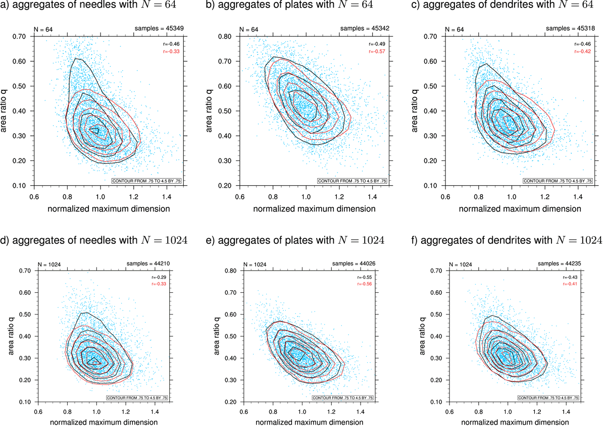
Figure 9
As Figure 9, but for the joint correlation of the normalized maximum dimension and the ellipsoidal area ratio q. The solid red lines are the parameterizations using Eqs. (26)–(28).
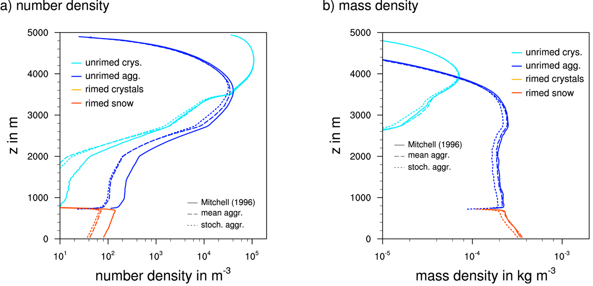
Figure 10
Vertical profiles of number and mass densities for the quasi-stationary state of 1D McSnow simulations (case 1). Super-particles are categorized as unrimed crystals, unrimed aggregates, rimed crystals, rimed aggregates, and liquid drops. The control simulation uses empirical aggregate geometry based on M96 (solid lines). The simulation using the new stochastically generated aggregates is represented by dotted lines. Dashed lines correspond to a simulation with the new aggregates, but using zero standard deviations, i.e., the deterministic mean aggregate snowflakes.
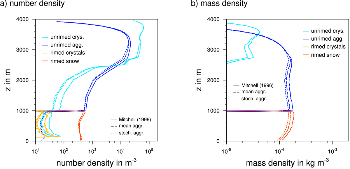
Figure 11
As in Figure 10, but for case 2 with a domain top at 4000 m and a nucleation layer in the uppermost 1500 m.
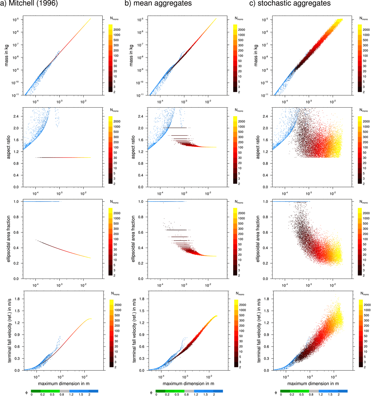
Figure 12
Scatter plots of the m–D, –D, q–D, and v–D relations for case 1 using empirical aggregates from M96 (left), mean aggregates (middle), and stochastic aggregates (right). All plots share the same x-axis showing the maximum dimension D. Color bars represent aspect ratio of monomers (green–gray-blue), aggregates are colored by monomer number N (brown–red–yellow). Fall velocities are adjusted to reference conditions hPa and K.
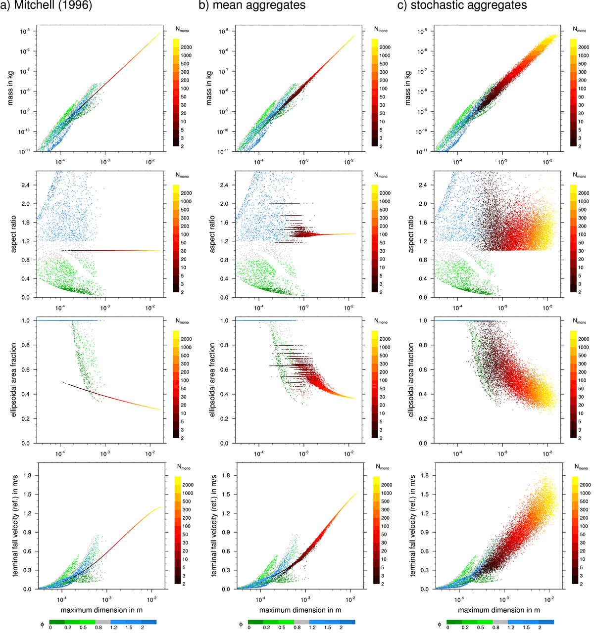
Figure 13
As in Figure 12, but for case 2 with a domain top at 4000 m and a nucleation layer in the uppermost 1500 m.
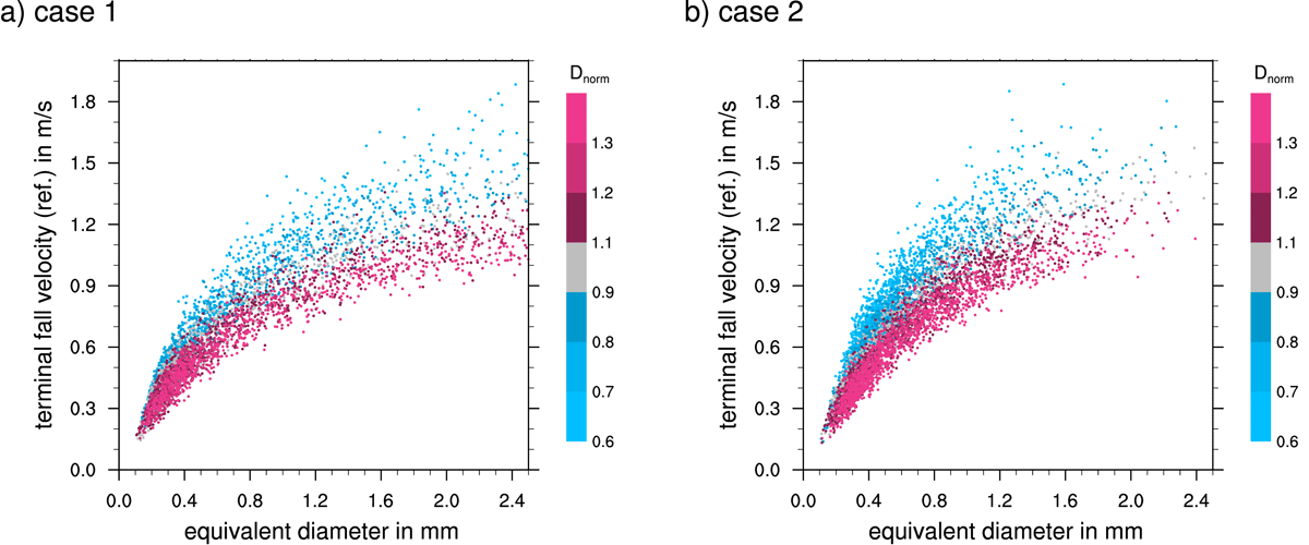
Figure 14
Scatter plot of terminal fall velocity of aggregate snowflakes as a function of equivalent diameter for case 1 (left) and case 2 (right). Colors indicate the normalized maximum dimension , with for elongated aggregates and for compact aggregates. Velocities are adjusted to 1000 hPa and 273.15 K.
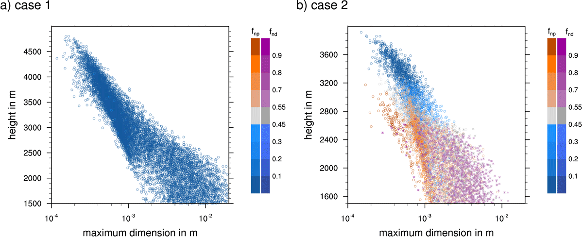
Figure 15
Scatter plot of aggregate snowflake size versus height. Colors indicate the number ratio of the binary habit mixture, with the dominant monomer habit shown as follows: blue for needles, orange for plates, and magenta for dendrites. Marker shapes denote mixed habit types: circles for needle–plate aggregates and stars for needle–dendrite aggregates. Data points have been thinned for clarity.
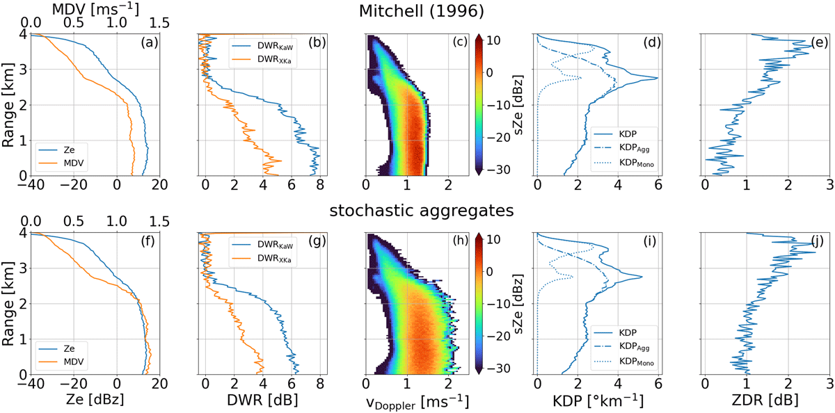
Figure 16
Radar forward simulations of case 2 using empirical aggregates from M96 (first row) and stochastic aggregates (second row). The first column (panels (a) and (f)) shows the radar reflectivity (Ze) and mean Doppler velocity (MDV) at Ka-band (35.6 GHz) and 90° elevation (zenith view). The second column (panels (b) and (g)) shows the reflectivity differences (in dB, commonly denoted as dual-wavelength ratio) at zenith between Ka- and W-band (94 GHz) and X (9.6 GHz) and Ka-Band. The third column (panels (c) and (h)) shows the zenith spectral reflectivity (sZe) at Ka-Band, the fourth column (panels (d) and (i)) shows the specific differential phase shift KDP at W-Band and 30° elevation, as well as the contributions of aggregates and monomers to the total KDP. The fifth column (panels (e) and (j)) shows the differential reflectivity ZDR at 30° elevation and W-Band.