
1 Introduction
Over the last few decades, data provided by meteorological satellites have become the predominant and one of the most valuable sources of information that is used in Numerical Weather Prediction (NWP) systems. This has been made possible thanks to the huge improvement of regional and global atmospheric forecast systems, data assimilation (DA), and forward models, together with the extensive technical progress on the Earth observation system and its continuity in time.
In particular, the importance of microwave satellite data to the forecast skill of NWP is well known. It has been shown in numerous studies that using microwave observations in the DA improves the forecasts for both global (Carminati et al., 2021; Chambon et al., 2023; Geer et al., 2017; Jiang et al., 2020; Lawrence et al., 2018; Li and Liu, 2016) and regional models (Schwartz et al., 2012; Storto and Randriamampianina, 2010; Xu et al., 2016; Zou, Qin and Weng, 2017). At higher latitudes, especially where geostationary satellites are of more limited use, and where the conventional observation network is sparse, an optimal use of microwave sounders on polar-orbiting satellites is crucial. Lawrence et al. (2019) highlighted the great importance of assimilating microwave sounding data over Polar regions while showing that the benefits are also propagated toward mid-latitudes. Recently, the study by Randriamampianina et al. (2021) demonstrated that microwave data have the largest relative impact on the upper-air humidity forecast skill, through both regional DA and lateral boundary conditions (LBCs). In addition, Laroche and Poan (2022) have shown the importance of data in the polar regions for global models, concluding that the joint impact of all Arctic satellite data on forecasts is two to four times larger than the impact of all conventional data in this area. Lindskog, Dybbroe and Randriamampianina (2021) have shown the importance of having polar microwave satellites evenly distributed throughout the day, so that the microwave satellite observations can be used in as many assimilation cycles as possible.
The current generation of microwave instruments on polar-orbiting platforms provides very valuable information on temperature and humidity profiles (via channels around 50 GHz and 183 GHz, respectively), which is commonly used to better constrain the initial conditions of the forecast. These instruments are also designed to observe the surface while measuring the emitted radiance at frequencies where atmospheric absorption is lower. These instruments are highly efficient and reliable; however, the time sampling is still far from optimal for regional systems. One reason is that microwave sounders are typically onboard heavy and costly platforms/programs together with several other instruments (such as infrared interferometers, scatterometers, and/or radio-occultation instruments, among others). These platforms carrying several instruments are expensive to build and to launch, so one alternative approach that is presently explored could be to use smaller and cheaper satellites.
In this context, it will be possible to deploy more small platforms in orbit and improve the temporal coverage of microwave observations over polar regions. In this regard, the European Space Agency (ESA) and the European Organisation for the Exploitation of Meteorological Satellites (EUMETSAT) are preparing to add a new operational observing system of microwave sounders. A constellation of six small satellites distributed in three orbital planes will be deployed and operated as part of the EUMETSAT Polar System program (EPS), under the name EPS-Sterna. The future constellation will provide an unprecedented amount of microwave data at very high sampling frequency, with a revisit time in the high latitudes of 60 minutes or less. The EPS-Sterna program is, at the time of writing, officially approved, which is finally allowing EUMETSAT to start the program. Such a program will be incredibly beneficial for both NWP and nowcasting activities. As a prototype for such a program, ESA has successfully launched the Arctic Weather Satellite (AWS) on 16 August 2024 (Eriksson et al., 2025). The commissioning phase officially ended with a successful outcome of the Commissioning Results Review on June 4, 2025, and the satellite is now operational. The original planned one year of operations, until August 2025, was recently extended by one year by ESA, and from 2026, EUMETSAT will take over and secure AWS operations until the end of 2029. European NWP centers have been involved in the process to provide feedback on the data quality.
Led by SMHI (the Swedish Meteorological and Hydrological Institute) and in collaboration with Finland, Denmark, and Norway, the ESA project Performance evaluation of AWS data (contract number 4000136511/21/NL/IA, https://arctic-weather-satellite.org/) was kicked off on 9 December 2021. It aimed at performing an early evaluation of the AWS data in the context of the regional NWP modeling systems of the Nordic countries. On-the-fly assimilation experiments using passive near-real time AWS data were run in a configuration that has been designed for that actual study.
Despite the significant positive impact that microwave observations introduce to the upper-air forecast skill, it was, however, mentioned in some recent studies that these observations are underused and have less impact in the Northern Hemisphere, particularly during winter (Bormann et al., 2017; Bormann, Lawrence and Farnan, 2019; Lawrence et al., 2019). This has been partly explained by the sub-optimal use of surface-sensitive observations over land and sea-ice. Unlike the Southern hemisphere, apart from Antarctica, which is mostly covered by “homogeneous” sea surfaces, the Northern hemisphere comprises large heterogeneous land surfaces (and sea-ice), covered by snow in winter at high latitudes. In these difficult conditions, where the model uncertainty is still large, the difference between the background estimate and the observation at surface-sensitive frequencies is often too large. Consequently, these observations are, most of the time, rejected by the quality check or even blocklisted.
Surface-sensitive channels measure a mixed signal coming from both the atmosphere and the surface. The latter is modeled in the radiative transfer by an effective skin temperature and an effective emissivity.
Over sea surfaces, several aspects facilitate the assimilation of low-peaking channels at microwave frequencies: (1) accurate surface emissivity models are available (Bormann, Geer and English, 2012; English et al., 2020; Liu, Weng and English, 2011), (2) skin temperature errors tend to be relatively small (less than 0.5 K), and (3) the contribution from the surface is smaller because its emissivity is lower (around 0.6–0.7).
Over land, snow, and sea-ice surface, however, the surface emissivity is higher (around 0.95) and more variable since it depends on the surface type/condition (forest, desert, humidity, snow, age of the ice, etc.), frequency, observation angle, among others. It is, still today, often set to a static value, or built on an old classification-based look-up table such as the one described in Weng, Yan and Grody (2001), assuming a surface that is flat and specular. The effective skin temperature, used in observation space, is another large source of error over land. Still based on the previous short-range forecast in some systems, its modelization is strongly simplified and does not take into account some crucial processes, such as the penetration effects.
Over the coast, the contribution from the surface is even more complex since the signal is coming from both the ocean and the continent. This mixed signal often leads to large departures between observations and model. Historically, the response has been to reject/discard observations where the portion of land in the pixel is higher than 50 %, without considering whether the observation or the model is primarily responsible for the resulting large departures.
The assimilation of satellite observations close to the surface has been (and it still remains) one of the most active areas of research for the last two decades. To better use surface-sensitive channels in the microwave band, Karbou et al. (2010a; 2010b) demonstrated that low-peaking microwave channels that received a large contribution from the surface can be successfully assimilated over land if the emissivity is adequately represented. They suggested using a window channel to retrieve the land surface emissivity and allocate the latter to adjacent sounding channels. In this way, the simulation of Brightness Temperature is improved, and a larger amount of observations can be assimilated to better constrain the atmospheric analysis. Over sea-ice and snow, the microwave surface emission is more variable and complex. Several assumptions in the modeling of this are likely to be inaccurate (Baordo and Geer, 2015; Bormann et al., 2017; Guedj et al., 2010; Karbou and Prigent, 2005; Matzler, 2005); however, these aspects will be covered in another document/article. The dynamic emissivity method has been used successfully in most global NWP centers such as the European Centre for Medium-Range Weather Forecasts (ECMWF) or Météo-France, and it is currently still operational, with some adjustments in most of them. For a few years, this approach has been implemented and operational in the regional model running over the Scandinavian and the Arctic domains.
The purpose of the present article is to evaluate the dynamic emissivity method in the context of the preparation for the AWS small satellite program (potentially EPS-Sterna). After this first introductory section, the second section presents the data and the methods used in this study. Expected benefits from AWS are also discussed in that section (since the data were not available yet). The third section details the results in terms of radiance simulation performances and validation scores against other observations. This paper aims to pave the way and discuss the future challenges that will be associated with the assimilation of the ESA/AWS and EPS-Sterna observing system.
2 Data and Methods
2.1 The HARMONIE-AROME model
In this study, a version (cycle 43h2.2) of the regional NWP system called HARMONIE-AROME (Hirlam and Aladin Research Model On Non-hydrostatic-forecast Inside Europe (Bengtsson et al., 2017)) has been used. This system is part of the code base of the IFS/ARPEGE (Integrated Forecasting System/Action de Recherche Petite Échelle Grande Échelle) and software system of ECMWF and Météo-France. It is developed and maintained in the framework of the international ACCORD (A Consortium for COnvection-scale modelling Research and Development (Fischer and Pottier, 2021)) consortium, in which 26 National Met Services are joining their scientific research efforts since January 2021 (http://www.umr-cnrm.fr/accord/). The three main components of HARMONIE-AROME are upper-air DA, surface DA, and the forecast model.
The model is non-hydrostatic with a dynamical core originating from the AROME-France model (Seity et al., 2011) based on the fully compressible Euler equation formulated in a terrain-following pressure-based sigma-coordinate system. The evolution of the equations is discretized in time and space using a semi-Lagrangian (SL) advection scheme on an A grid and a semi-implicit two-time-level scheme, with spectral representation of most prognostic variables based on a double Fourier decomposition. The model physics comprises numerical schemes and parameterizations for radiation, clouds and cloud microphysics, turbulence, and convection. Deep convection is explicitly resolved at the typical model resolution, while shallow convection and surface fluxes are represented through parameterizations. The surface is handled separately in the SURface EXternalisée (SURFEX) scheme (Masson et al., 2013). It includes a three-layer version of the Interaction Soil Biosphere Atmosphere (ISBA) force-restore scheme (Boone, Calvet and Noilhan, 1999) as well as a single-layer snow model (Douville, Royer and Mahfouf, 1995). Using the optimal interpolation technique, the surface humidity and temperature are initialized with observations at 2 m height. Similarly, the snow depth observations are interpolated to initialize the snow model. The sea-surface temperature is taken from the ECMWF forecast system (making use of Operational Sea Surface Temperature and Sea Ice Analysis (OSTIA: Donlon et al., 2012), the Ocean and Sea Ice Satellite Application Facilities (OSI-SAF: Tonboe et al. (2016) is providing sea-ice concentrations and the sea-ice temperature is described by a prognostic equation in the Simple Sea Ice Scheme (SICE: Batrak, Kourzeneva and Homleid, 2018). The surface DA is done in a totally separate step from the upper-air assimilation, so that they are not strongly coupled together.
The default HARMONIE-AROME atmospheric DA methodology is based on a 3-dimensional variational (3D-Var) scheme (Fischer et al., 2006). A 4-dimensional variational (4D-Var) approach has also been developed as a potential candidate for future operational use. In this study, both 3D-Var and 4D-Var are considered. HARMONIE-AROME 4D-Var uses a multi-incremental approach (Courtier, Thépaut and Hollingsworth, 1994). Non-linearities are handled by a sequence of re-linearizations, called outer loop iterations, which communicate through files that either contain meteorological fields, observations or parameters. Here, we apply two consecutive outer-loop iterations by carrying out the first outer-loop iterations at a lower horizontal resolution (one sixth of full model resolution), followed by the second outer-loop iteration at a higher resolution (one third of full model resolution). This multi-resolution approach allows for reduced computational cost during the minimization of the cost function by first handling larger scales and then incrementally introducing finer-scale features. The main advantages of the 4D-Var procedure as compared to 3D-Var is the use of observations at their appropriate time and the use of a simplified version of the forecast model within the assimilation procedure (Barkmeijer et al., 2021). In 4D-Var, observational data are sorted into 10 distributed time slots within the assimilation time window ranging from –2 h to 1 h relative to the assimilation main times at 00, 03, 06, 09, 12, 15, 18, and 21 UTC. For 3D-Var, there is only one time slot, and the assimilation time window ranges from –1.5 to +1.5 h. However, for satellite data, we here use operational data with a cut-off time of 1 h and 15 min. Data thinning-procedures are applied per time slot to alleviate the effects of spatially correlated observation errors currently not explicitly represented (Bormann and Bauer, 2010). This means that 4D-Var allows for the use of a substantially larger amount of satellite observations.
The climatological background error covariances used in this study were estimated from an ensemble of forecast perturbations obtained by dynamically downscaling ECMWF Ensemble of Data Assimilations (EDA) fields to convection-permitting scales. The EDA-derived ensemble forecasts were subsequently remapped in both the horizontal and vertical to the native grid and vertical discretization of the HARMONIE-AROME 2.5 km configuration, and used as initial conditions for high-resolution, non-hydrostatic integrations of the limited-area model (Berre, 2000; Bonavita, Isaksen and Hólm, 2012; Brousseau et al., 2012).
A wide range of observations are presently assimilated in the operational suite from conventional measurements (synop, buoys, ship, radiosonde, and aircraft), satellite data (infrared and microwave radiances, scatterometer winds, and atmospheric motion vectors), Global Navigation Satellite System (GNSS, Lindskog et al., 2017), and from weather radar winds and reflectivities (Ridal, Sanchez-Arriola and Dahlbom, 2023). Prior to the assimilation, observations are (1) projected to the model state using an observation operator (i.e., the RTTOV radiative transfer model for radiances), (2) bias corrected (using a Variational Bias Correction (VarBC; Auligné, McNally and Dee, 2007; Benáček and Mile, 2019; Dee, 2005), and (3) thinned and quality checked.
In this study, the model was run over a domain covering the Nordic region (see Figure 1) using a 2.5 km grid point resolution, with 65 vertical levels. This is the operational domain of MetCoOp, which is the Meteorological Cooperation on Operational NWP between the Finnish, Norwegian, Swedish, Estonian, and Latvian National Meteorological Services (FMI, Met Norway, SMHI, ESTEA and LVGMC). The initial fields and LBCs are hourly forced by the ECMWF/IFS Forecasting System. Global model information is also used to replace larger-scale information in the background state with lateral boundary information (Müller et al., 2017). The idea is to make use of high-quality large-scale information from the ECMWF global fields, in the MetCoOp analysis. In particular, temperature and wind components are mixed while humidity is excluded from this process. This exclusion of humidity prevents a dry bias in HARMONIE-AROME that would result from different model physics between HARMONIE-AROME and ECMWF, though it may create slight inconsistencies between temperature and humidity fields (Schönach, Eresmaa and Järvinen, 2025). A more refined method, as described by Guidard and Fischer (2008) as well as by Dahlgren and Gustafsson (2012), would be to incorporate the global host model field as one additional term in the cost function to be minimized in the upper-air variational DA.
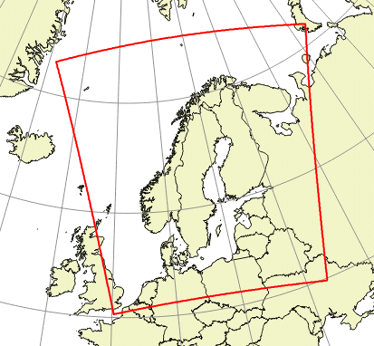
Figure 1
The MetCoOp domain.
2.2 Microwave radiance observations
The Advanced Microwave Sounding Unit (AMSU-A) and the Microwave Humidity Sensor (MHS) sounders were operating on board the American National Oceanic and Atmospheric Administration (NOAA-15, -18, and -19) and the European Meteorological Operational (Metop-A, -B, and -C) series of polar-orbiting satellites. On a global scale, sun-synchronous polar-orbiting platforms permit the generation of a near-global data coverage twice/day. On a regional scale, the data coverage is not uniform in time and space over the domain of interest. As shown in Figure 2, the amount of available radiance data over the MetCoOp domain significantly depends on the time and the day. In February 2021 when the highest amount of AMSU-A and MHS instruments were operational, one can note that 09 UTC, 18 UTC, and 21 UTC benefit from the best coverage. There are no/few data available at 00 UTC and 03 UTC, and a partial coverage at 12 and 15 UTC. The more recent operational version has been closing the gap since then while assimilating data from the Advanced Technology Microwave Sounder (ATMS) onboard the Suomi NPP, NOAA-20, and NOAA-21 satellites and the Micro-Wave Humidity Sounder (MWHS)-2 onboard the FY-3 series of satellites.
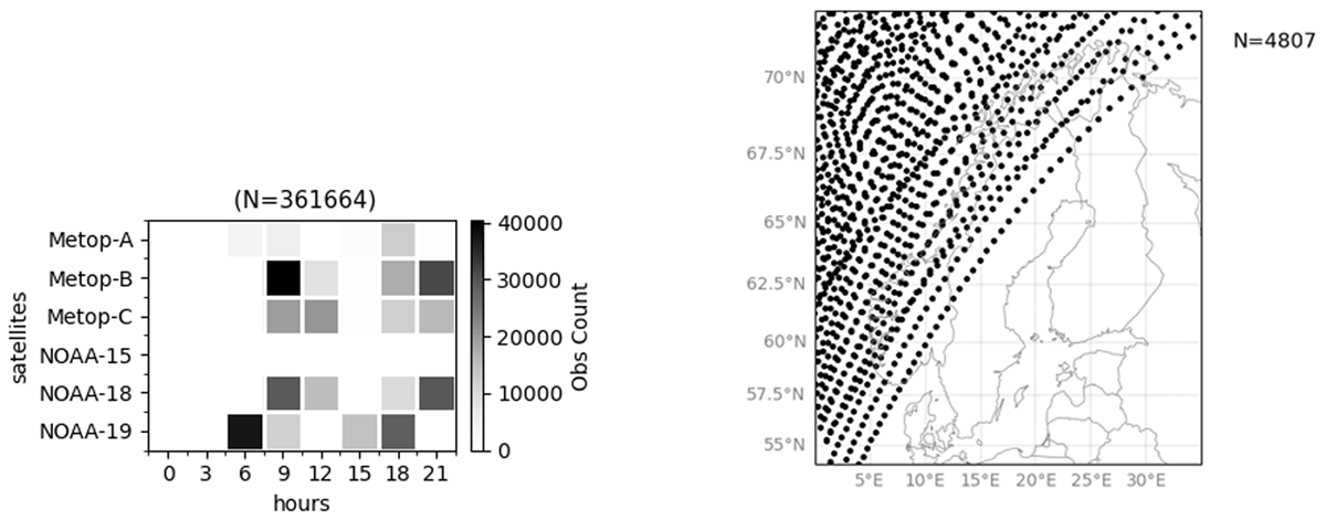
Figure 2
Amount of available AMSU-A radiance observations (all channels) over the MetCoOp domain on the 10 February 2021, for each satellite and assimilation window (left panel). Map of available observations at 12 UTC (right panel).
The two instruments and AWS are using a cross-track scanning technique: 30 positions (from –48° to +48° with respect to nadir) covering a swath of 2250 km for AMSU-A, 90 positions (from –49.5° to +49.5°) covering a swath of 1650 km for MHS, 145 positions (from –55° to +55°) with a swath of approximately 2000 km (Albers, Emrich and Murk, 2023; Lagaune, Berge and Emrich, 2021) for AWS. At nadir, the AMSU-A (MHS) instrument footprint corresponds to a circle of diameter approximately 48 km (16 km). For AWS, the resolution is slightly better with footprints below 40 km at 50 GHz temperature channels and around 10 km for the 180 GHz group of humidity channels (Eriksson et al., 2025).
AMSU-A is designed for atmospheric temperature sensing, the MHS sounder is used for humidity probing, and AWS will combine both capabilities. The AMSU-A instrument provides measurements at 15 frequencies, which include 12 frequencies near the oxygen absorption band (50–60 GHz). MHS makes measurements at 3 frequencies close to the strong water vapor absorption line at 183.31 GHz and 190.31 GHz. The three instruments also have some “window channels” which give measurements sensitive to the surface (23.8, 31.4, 50.3, 89, and 157 GHz). Onboard the AWS platform, the microwave sounding instrument will provide measurements in 19 channels, both in humidity and temperature, including 5 that are common with AMSU-A and 3 that are equivalent to MHS. AWS also includes soundings in the 325 GHz band, for the first time providing observations in the sub-mm range from space. Together with the 183 GHz channels, these new bands are expected to improve the disentangled retrieval of humidity and cloud ice, useful in many applications, including clear-sky assimilation (Kaur et al., 2021). The channel characteristics of AMSU-A and MHS are given in Table 1 as well as common/equivalent features to AWS (following Eriksson et al., 2025; Table 4).
Table 1
AMSU-A and MHS characteristics, with corresponding equivalent AWS channels. Observe that we here use a running number from 1 to 19 for the AWS channel ids, as it is used in RTTOV, see, e.g., the WMO OSCAR database at https://space.oscar.wmo.int/instruments/view/mwr_aws.
| INSTRUMENT | CHANNEL IDX | FREQUENCY (GHz) | SENSITIVITY | AWS (CHANNEL IDX) |
|---|---|---|---|---|
| AMSU-A | 1 | 23.8 | surface | no |
| 2 | 31.4 | surface | no | |
| 3 | 50.3 | surface | yes (1) | |
| 4 | 52.8 | temperature | yes (2) | |
| 5 | 53.596±0.115 | temperature | yes (4) | |
| 6 | 54.4 | temperature | yes (5) | |
| 7 | 54.9 | temperature | yes (6) | |
| 8 | 55.5 | temperature | yes (7) | |
| 9 | ν=57.290 | temperature | yes (8) | |
| 10 | ν±0.217 | temperature | no | |
| 11 | ν±0.322±0.048 | temperature | no | |
| 12 | ν±0.322±0.022 | temperature | no | |
| 13 | ν±0.322±0.010 | temperature | no | |
| 14 | ν±0.322±0.0045 | temperature | no | |
| 15 | 89 | surface | yes (9) | |
| MHS | 1 | 89 | surface | yes (9) |
| 2 | 157 | humidity | eq* (10, 165.5 GHz) | |
| 3 | 183±1 | humidity | eq* (15, 182.311 GHz) | |
| 4 | 183±3 | humidity | eq* (13, 180.311 GHz) | |
| 5 | 190.311 | humidity | eq* (11, 176.311 GHz) |
[i] eq*: equivalent channels to AWS.
Figure 3 shows the weighting functions for AMSU-A, MHS, and AWS channels calculated for a standard sub-Arctic atmosphere, in winter, at nadir using the RTTOV radiative transfer model. The weighting functions show the relative contribution of each atmospheric layer to the measured radiance in terms of humidity and temperature. As illustrated in Figure 3, high-peaking channels (such as AMSU-A channel 8, which is equivalent to AWS channel 7) show the peak of their weighting function very high in the atmosphere (around 180 hPa). On the contrary, at window channels, where the atmosphere is relatively transparent, the weighting functions have their maximum at the surface, being almost not sensitive to atmospheric humidity and temperature. Low-peaking channels (such as MHS channel 5, which is equivalent to AWS channel 11) show a maximum closer to the surface (around 900 hPa) and receive a mixed signal from the surface and the atmosphere. For all these channels, it is important to accurately model the surface emission (emissivity and surface temperature) to correctly separate its effect from the atmospheric one and simulate a realistic radiance.
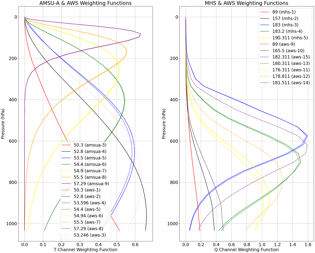
Figure 3
AMSU-A and MHS (plain lines) together with AWS (dashed lines) weighting functions for a 64-level reference profile at nadir over sub-Arctic for temperature channels (left panel) and water vapor (right panel) channels.
Presently, within the preprocessing chain of HARMONIE-AROME, the RTTOV radiative transfer model is fed by the following surface information: 1) surface temperature is a short-range forecast provided by SURFEX and OSTIA (see Section 2.1), and 2) the surface emissivity uses FASTEM-4 over sea surfaces and, over land, either a classification-based emissivity scheme (Grody, 1988; Weng, Yan and Grody, 2001) over land for AMSU-A or a constant value for MHS:
exposed dry land
exposed moist land or light snow cover
exposed deep snow cover if K then else
exposed very deep snow cover if K then else
Because the uncertainties in land surface temperature and emissivity are very high, the strategy has been to reject/discard surface-sensitive observations where large systematic departures exist, without considering whether the observation or the model is primarily responsible. In the next sections, we explore a methodology to overcome this limitation and enable the use of more low-peaking channels in the microwave to potentially improve the forecast skill of our regional system.
2.3 The dynamic emissivity method over land and sea-ice
Karbou et al. (2010a) and Karbou, Rabier and Prigent (2014) demonstrated that microwave surface-sensitive channels can be assimilated over land and sea-ice with an adequate description of the surface emissivity.
The emissivity () is the ratio of energy emitted from a natural material to the one from an ideal black body at the same temperature. It varies with the frequency, with the surface type and also with the observation scan angle. Together with land surface temperature (Ts), an accurate surface is desired for better simulations of surface-sensitive microwave radiances.
For a given frequency and at observation zenith angle , the Brightness Temperature Tb can be expressed through the integrated radiative transfer equation in the Rayleigh–Jeans approximation for a non-scattering plane-parallel atmosphere by:
where represents the surface emissivity, Ts, , and are the surface temperature, the atmospheric downwelling and upwelling Tb, respectively. The net atmospheric transmissivity is expressed as a function of the atmospheric opacity and the observation zenith angle . H is the top-of-the-atmosphere height.
Instead of using the default HARMONIE-AROME emissivity over land, one can use an “effective” surface emissivity, derived following (Karbou and Prigent, 2005). Assuming (1) a non-scattering and plane-parallel atmosphere, (2) a specular reflection over the surface in , (3) the medium emits at the temperature of the surface skin, and (4) the variability of emissivity with frequency is low, the emissivity can be retrieved, at a window channel, and allocated to adjacent (in frequency space) sounding channels, reversing the radiative transfer equation 1 by:
The emissivity is retrieved at each observation point, prior to the Tb simulation. Together with the Ts provided by the HARMONIE-AROME background, emissivity retrievals are used over land to simulate the Tb in a dynamical way (i.e., updated continuously) and in a consistent way with the instrument characteristic (resolution, geometry, etc.). In this study, the emissivity retrieved at AMSU-A channel 3 (MHS channel 1) is allocated to AMSU-A channels 4 to 9 (MHS channels 3 to 5). The emissivity at AMSU-A channels 1 and 2 (MHS channel 2) has been retrieved too, even though it is not used further in the assimilation process.
Also, when the atmospheric transmission is lower than 0.5, the dynamical estimation of emissivity is not performed to avoid too noisy emissivity retrievals. It regards less than 0.1 % of the cases since the atmospheric transmittance at the surface is high at these latitudes and frequencies (see Table 2).
Table 2
Mean (standard deviation) of atmospheric transmittance at surface for radiances at AMSU-A and MHS window channels (data from 10 February 2021-09 UTC and 10 June 2021-09 UTC).
| AMSU-A CHANNEL 3 | MHS CHANNEL 1 | MHS CHANNEL 2 | |
|---|---|---|---|
| Summer | 0.66 (0.03) | 0.77 (0.06) | 0.46 (0.11) |
| Winter | 0.66 (0.03) | 0.90 (0.02) | 0.84 (0.05) |
In this case, emissivities from a monthly emissivity atlas are used over land surfaces or static emissivity is taken for sea-ice. Atlases were kindly provided by Météo-France. These monthly maps were computed using AMSU-A and MHS observations from 2015 together with short-range forecast of the French global ARPEGE model. Atlases are also available on the EUMETSAT NWP SAF website: https://nwp-saf.eumetsat.int/site/software/rttov/download/. In the context of this study, the cloud/rain contamination of microwave observations is likely to occur and could explain part of the variability of the emissivity, resulting in larger observation departures from first guess or from analysis.
Another limitation of the methodology concerns snow-covered land and sea-ice surfaces. In particular, the assumptions (2), (3), and (4) could be questionable in some situations (Baordo and Geer, 2015; Bormann et al., 2017; Guedj et al., 2010 among others). In this paper, sea-ice emissivity at MHS frequencies has been retrieved following (Karbou, Rabier and Prigent, 2014). The emissivity is retrieved at channel 1 (89 GHz) and propagated at channel 2 (157 GHz) using a linear regression method as follows:
where is the extrapolated emissivity at channel 2 (157 GHz) computed using the retrieved emissivity at channel 1 () and the difference between observed Brightness Temperature at channels 1 and 2 ( and the surface skin temperature from a short range forecast of HARMONIE-AROME (Ts).
Also, the level of uncertainties on the retrieval can be very high over heterogeneous pixels that comprise, for example, a portion of land with high emissivity mixed with a portion of open-sea where the emissivity is significantly lower. In order to overcome that limitation and reduce these representativeness errors, a new methodology called the “footprint operator” is being developed and tested at MET Norway. While this method is being optimized and validated, the heterogeneous pixels (i.e., coast) will be blocklisted.
2.4 Benefits and expected challenges with AWS
One expected challenge with respect to AWS is that, in Level 1b, a raw observation measurement made at the same time points to four different locations. As shown in Figure 4 and explained and discussed in more detail by Rydberg (2025), Albers, Emrich and Murk (2023), and Eriksson et al. (2025), the instrument design implies that the geolocation of observations will be slightly shifted depending on the frequencies in terms of latitude and longitude. There will be four groups of frequencies (i.e., “Horn” in Figure 4): Horn-1: 54 GHz, Horn-2: 89 GHz, Horn-3: 183 GHz, and Horn-4: 325 GHz. As mentioned in the previous section, the dynamic emissivity method uses a window channel to retrieve the surface emissivity, which is in turn allocated to an adjacent channel in terms of frequency. Horn-1 includes both the 50.3 GHz window channel and the sounding channels for temperature probing at the same location. However, sounding channels from Horn-3 (183 GHz’s) should use the emissivity retrieved at the 89 GHz channel from Horn-2. Furthermore, there are plans to use 325 GHz channel data for a refined cloud filtering of 183 GHz radiances. This will be somewhat complicated by the different locations of 183 and 325 GHz radiances.
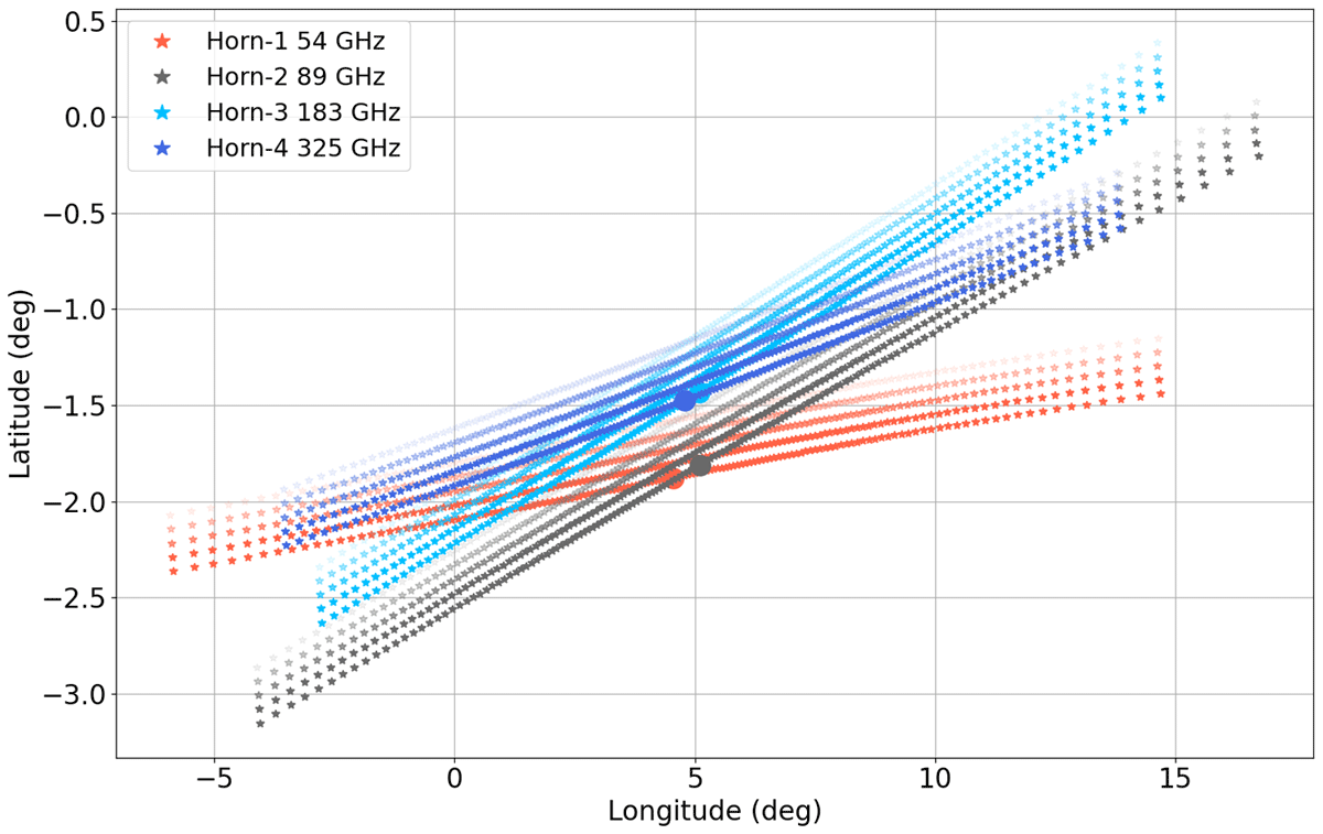
Figure 4
Expected geolocation lat/lon shift of observation as seen from the boresight locations on ground for five consecutive scan lines of all four AWS feed horns. Based on real data 4 May 2025, around 22:15 UTC. Scan position 73 (the middle position—not identical to the sub-satellite track) of the first scan line of each feed horn is marked by a large dot.
An obvious approach to overcome this apparent obstacle is to take advantage of the dense sampling (and in particular for Horn 1 and 2 the high oversampling) and apply a remapping of the data prior to presenting it to the assimilation system as Level 1c, e.g., as provided in Rydberg (2025). One could, for example, relocate all data to the positions of the 183 GHz radiances. The effects of having interpolated the window channel at 89 GHz data to be used for low-peaking channels remain to be investigated. There might be some potential detrimental effects close to coastlines or in situations with strong and rapid horizontal variations.
Another challenging aspect is that the satellite observations are assumed to be spatially representative for the regional numerical model. In fact, representation error might exist when unobserved scales and processes of the high-resolution model are constrained by coarse-resolution satellite observations. The application of a footprint observation operator can result in a more optimal use of AWS-like satellite data, correcting only the relevant scales in high-resolution DA. There are particular examples of footprint operator implementations (Buehner et al., 2013; Carrieres et al., 2017; Mile, Azad and Marseille, 2022; Mile et al., 2021); however, their operational usage is not common so far. Such representation error exists in radiance DA as well and the importance of the footprint representation has been identified, for example, in the use of infra-red satellite observations (Duffourg et al., 2010).
For AWS radiances, an appropriate footprint operator might help to better exploit the observations by taking into account the spatial representativeness of the radiance measurements in high-resolution HARMONIE-AROME assimilation system. For instance, the quality control is a key issue where the footprint operator can be efficiently used to detect spatial inconsistencies. It might be important with Level 1c but most probably with Level 1b radiances, playing a role in the geolocation of the observation. Additionally, when Level 1c data is assimilated, the footprint observation operator can help to better calculate model-equivalent departures and to remove the representation error over complex or mixed surface scenes. A prototype microwave AMSU-A footprint operator was developed and tested by Mile, Guedj and Randriamampianina (2024). Figure 5 shows an example of one AMSU-A scanline where mixed surfaces and sub-footprint variability is considerable, a case where the use of the footprint operator is expected to be beneficial.
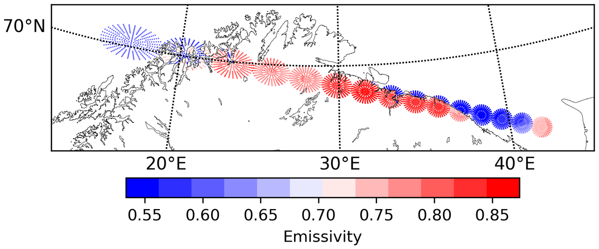
Figure 5
IFOV representation for a single AMSU-A scanline and using a microwave radiance footprint operator. The retrieved surface emissivity is plotted inside the IFOV, i.e., footprint area indicating the heterogeneous surface conditions over the MetCoOp domain.
3 Results
3.1 Experimental setup
To assess the forecast impact of adding the surface-sensitive microwave sounding data, a set of assimilation trials was conduced with the HARMONIE-AROME system for 6 weeks (from 15 January to 28 February 2021). This month was chosen because it was one of the coldest periods with one of the largest areas covered by snow and sea-ice during recent years over our domain. During this period, three Metop platforms were operating simultaneously, maximizing the availability of AMSU-A and MHS radiances. However, since Metop-A was approaching its “End Of Life” and had drifted considerably from its initial orbiting trajectory, it was decided to discard this platform from all DA experiments. The experiments are run eight times per day with a forecast length of 36 hours for the main cycles (00, 06, 12, and 18 UTC) and shorter catch-up runs of 3 hours for the intermediate cycles. In order to highlight the impact of low-peaking microwave observations, only a subset of the entire observing system is assimilated: conventional observations together with radiances from the IASI hyperspectral sounder and the two microwave sounders AMSU-A and MHS. Data from both Metop and NOAA’s platforms are actively assimilated.
The first baseline experiment is a close version of the operational 3D-Var MetCoOp system (cycle 43) as it was when the ESA/AWS project started (in January 2022). A second baseline has been built in a 4D-Var framework, which could be a candidate for the next operational suite. Both baseline experiments are called ctl-3D-Var and ctl-4D-Var, respectively. These two baseline configurations have not been designed to be compared against each other in this study. Each of them separately aims to be a reference for another experiment in which the low-peaking channels are used. AMSU-A channel 5 is blocklisted over all surfaces in these baseline configurations. MHS channel 5 is blocklisted over 55 latitude North. The surface emissivity is set to default (see next section for more details).
Associated with each baseline experiment, two additional experiments have been set up in which the microwave low-peaking channel 5 of AMSU-A and MHS are actively assimilated over land and sea-ice using the dynamic emissivity method (called ldyn-3D-Var and ldyn-4D-Var further). Since these experiments make use of two additional channels that were blocklisted in the MetCoOp system (see Figure 3), a preliminary experiment has been run beforehand to provide a warm start to the VarBC bias correction scheme.
To go further into details in the analysis, ldyn-3D-Var and ldyn-4D-Var were run without the assimilation of low-peaking channels, but keeping the dynamic emissivity method active. These two configurations are called nolwp-3D-Var and nolwp-4D-Var. A summary is presented in Table 3.
3.2 Simulation of microwave radiances and the dynamic emissivity method
3.2.1 Evaluation of emissivity retrievals
In this section, the retrieved emissivity from ldyn-3D-Var and ldyn-4D-Var is compared with (1) the default surface emissivity used in operation (as in ctl-3D-Var and ctl-4D-Var) and (2) the atlases provided by Météo-France and used as back-up emissivity in ldyn-3D-Var and ldyn-4D-Var. In addition, the emissivity is then used to simulate Brightness Temperature. To increase the robustness of the statistics, all available data are considered in this session (i.e., not only active data), except specified otherwise.
Using the RTTOV radiative transfer model together with outputs from short-range atmospheric forecast, the surface emissivity at AMSU-A channel 3 (50 GHz) and MHS channel 1 and 2 (89 GHz and 157 GHz) have been retrieved every 3 hours over all surfaces (in the ldyn-3D-Var and ldyn-4D-Var experiments). The emissivity back-up atlases have been introduced in ldyn-3D-Var and ldyn-4D-Var experiments. The default emissivity has been extracted from ctl-3D-Var and ctl-4D-Var. Sea-ice observations and land snow-covered observations are identified with a basic test on the skin surface temperature from the background (Ts < 273 K).
Overall, Figure 6 shows that the default land surface emissivity maps at AMSU-A channel 3 (50 GHz) over the MetCoOp domain are around 10 % lower compared to the back-up emissivity atlas on 10 February at 09 UTC. The retrievals seem closer to the back-up emissivity atlas (around 1 %). The retrievals over open sea-surfaces seem slightly higher than the one obtained from FASTEM model. However, the system is, by default, using FASTEM, and the surface emissivity of open-sea surfaces is out of the scope of this article.
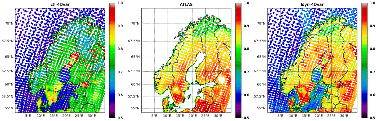
Figure 6
Default (which would have resulted from the previously used system) land surface emissivity map (left), backup atlas emissivity maps (middle panel) compared to a “snapshot” of the dynamical retrieved emissivity (right panel) at AMSU-A Channel 3 (50 GHz) on 10 February 2021, 09 UTC.
As shown in Figure 7a, the land surface emissivity retrieved over snow-covered observations describes large differences with the default scheme (on average 0.15). The back-up emissivity atlas is very consistent with the retrievals. Over snow-free land surfaces, the differences are significantly reduced and the three datasets agree slightly more (Figure 7b).
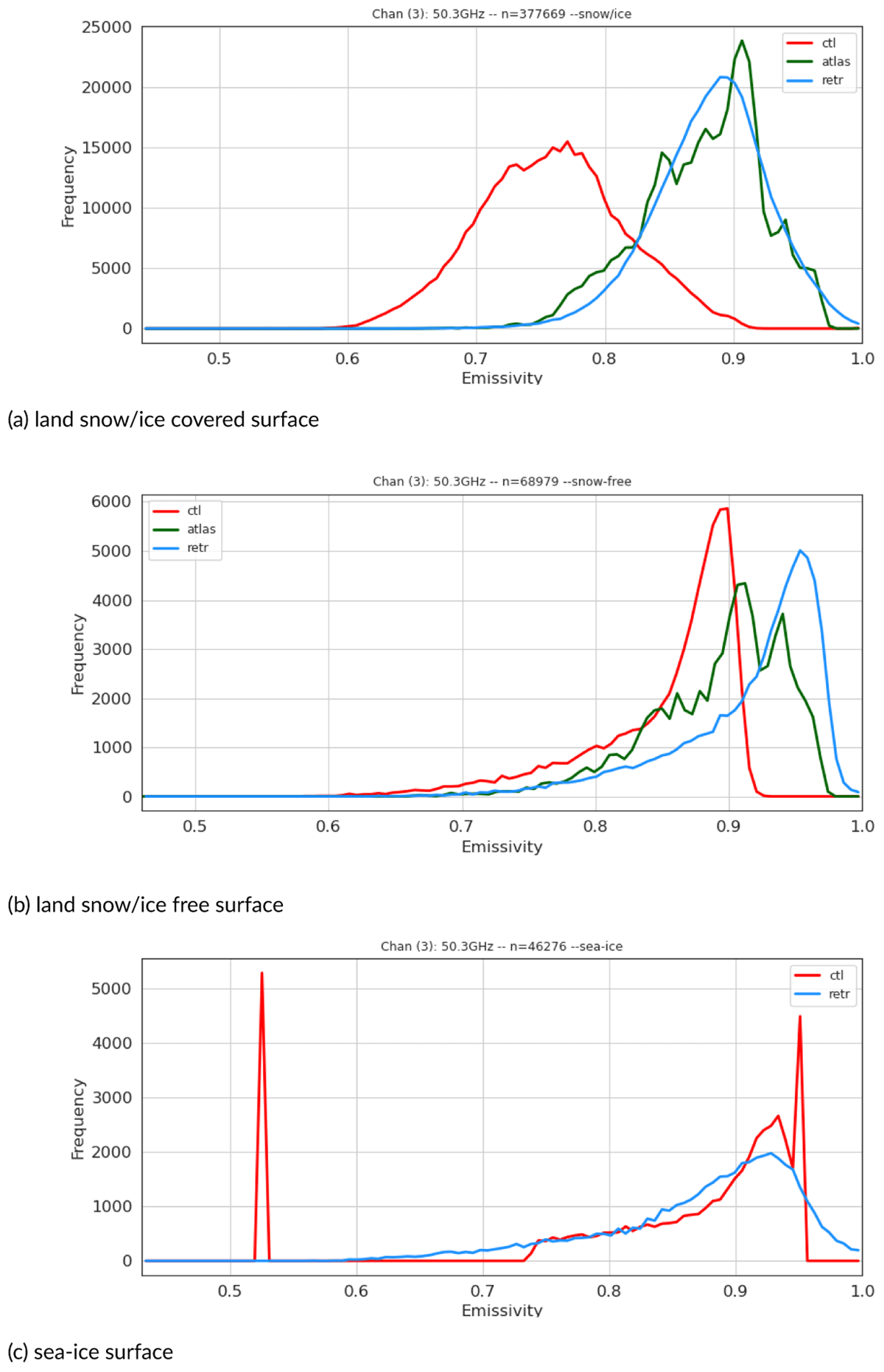
Figure 7
Histograms of land and sea surface emissivity at AMSU-A channel 3 (50 GHz) over (a) snow-covered land surface, (b) snow-free land surfaces, and (c) sea-ice in February 2021. HARMONIE-AROME default emissivity (ctl-4D-Var) in red, dynamical retrievals (ldyn-4D-Var) in blue, and averaged ATLAS emissivities in green.
Over sea-ice, the evaluation is more challenging. First, there is no pre-computed atlas available from the 2015 database. Second, the identification of full sea-ice observations or mixed ocean/sea-ice using the single criterion of the model skin temperature threshold (Ts < 273 K) is strongly sub-optimal. In Figure 8a, a comparison between the constant default emissivity of 0.95 hardcoded in ctl-4D-Var for MHS channel 1 (89 GHz) and the emissivity retrieved in ldyn-4D-Var configuration is given on a specific case (10 February 09 UTC). In the latter, the average emissivity is about 0.87 with a standard deviation approaching 0.06. Compared to the static sub-optimal value that is used in the ctl-4D-Var, one can see the benefit of using ldyn-4D-Var to capture more closely the variability of sea-ice emission.
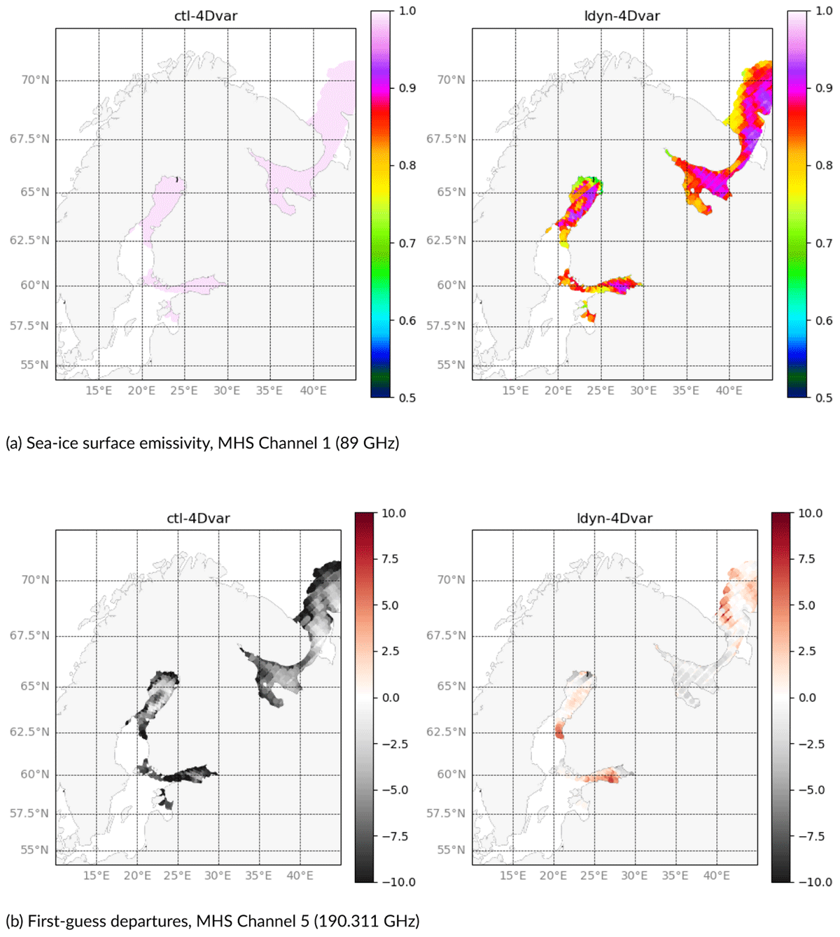
Figure 8
(a) Sea-ice surface emissivity maps at MHS Channel 1 (89 GHz) on 10 February 2021-09 UTC. HARMONIE-AROME static default emissivity (ctl-4D-Var) on the left, compared to the retrieved emissivity (ldyn-4D-Var) on the right. (b) First-guess departures at MHS channel 5 (190.311 GHz) with HARMONIE-AROME static default emissivity (left panel), and emissivity retrievals (right panel) used as input to RTTOV.
To evaluate the impact of using the retrieval instead of the default emissivity value, the RTTOV radiative transfer model has been run a second time to simulate the Brightness Temperature of adjacent sounding channels of each instrument over land and sea-ice. As input, the model used atmospheric 3h-First-guess profiles and surface temperature from HARMONIE-AROME together with either the emissivity from (1) the ctl-4D-Var and (2) the retrievals at the corresponding window channel (ldyn-4D-Var).
Focusing on sea-ice surfaces, Figure 8b gives an example of the benefit of using retrieved (and interpolated) emissivity instead of the static default emissivity to simulate MHS channel 5 (190 GHz) observations for one specific case (10 February 2021 – 09 UTC). A large average negative bias (–6.6 K) in the ctl-4D-Var has been reduced to +1.5 K bias.
Figures 9 and 10 show the frequency histograms of observed (OBS) versus simulated Brightness Temperature of AMSU-A and MHS sounding channels over various surfaces (snow or snow-free land and sea-ice or open sea). The use of the dynamic emissivity in ldyn-3D-Var instead of the default emissivities in ctl-3D-Var improves the quality of the Brightness Temperature simulations over all surfaces for low-peaking channels that received a significant contribution from the surface. As expected, the impact is quasi-neutral on higher-peaking channels (AMSU-A channels 6 and 7 as well as MHS channel 4). A slight degradation of simulated Brightness Temperature at MHS channel 3 over sea-ice can be observed.
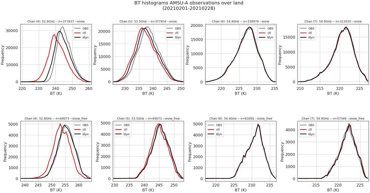
Figure 9
Histograms of observed (OBS) in gray and simulated Brightness Temperature (BT) in over land (snow or snow-free) surfaces of AMSU-A sounding channels using in the ctl-3D-Var in red or ldyn-3D-Var in black configurations. Statistics use data from February 2021 over the MetCoOp domain.
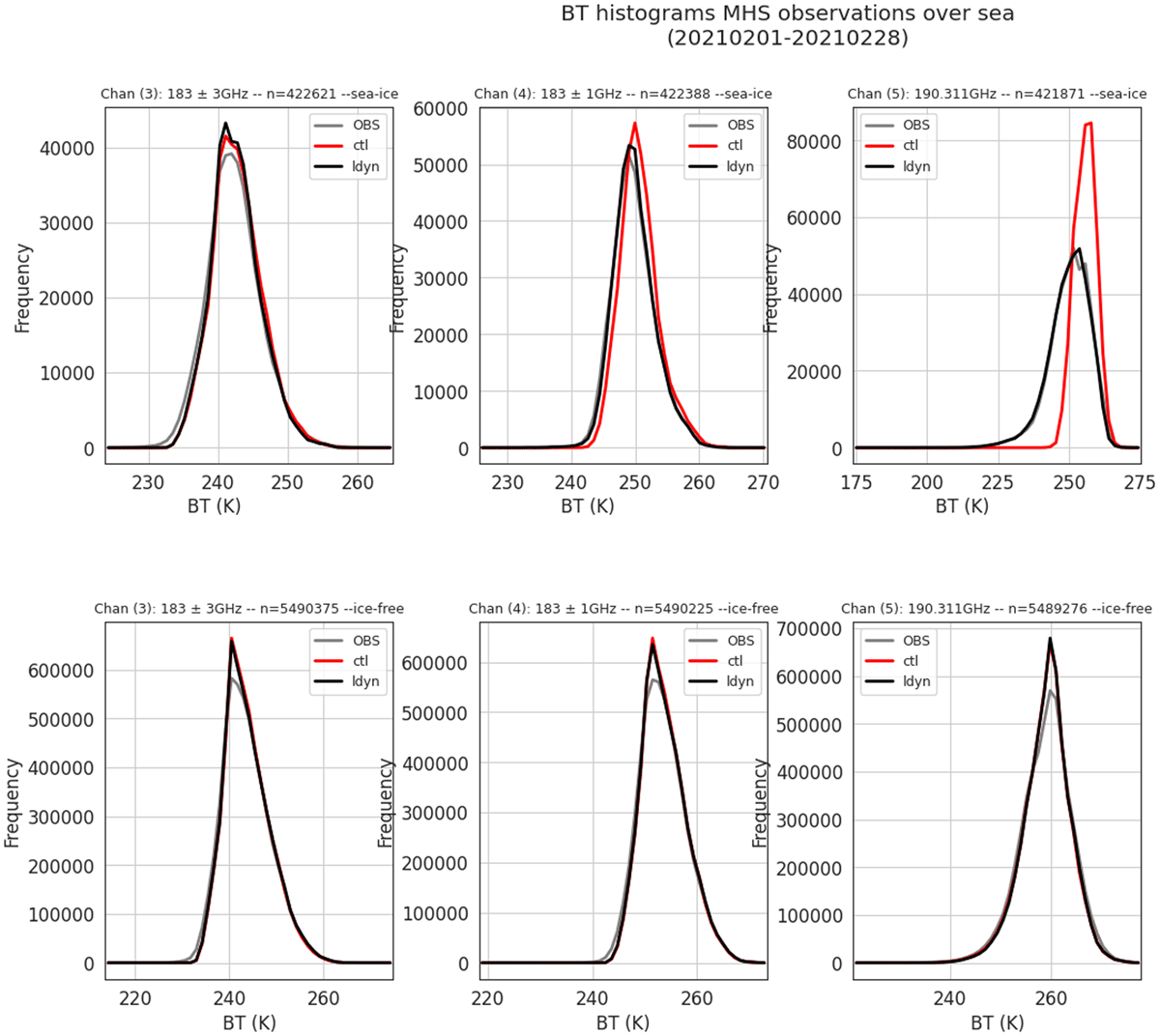
Figure 10
Same as Figure 9 but for MHS sounding channels over sea (sea-ice or open sea) surfaces.
Even if the Brightness Temperature simulations at low-peaking channels have been improved with the use of retrieved emissivity instead of the static one, a residual bias remains. The next session presents the benefit of using the variational bias correction before assimilating the radiance observations.
3.2.2 Monitoring and bias correction
In this subsection, the satellite radiances are monitored for systematic departures (or biases) relative to the assimilation system of HARMONIE-AROME. Time series of First-guess departures to observations are evaluated. It is expected that the bias in microwave radiances varies in time (e.g., diurnal or seasonal), in space (e.g., geographically and with air-mass too), as well as with the satellite instrument specification (e.g., with the scan position of the satellite instrument and with the orbital position of the satellite). It is commonly assumed that the bias is coming from several sources: (1) from the satellite instrument (i.e., calibration, degradation, environmental effects), (2) from the radiative transfer model physics and assumptions, (3) from the pre-processing of observations (cloud/precipitation screening/level 2 products) and/or (4) from the NWP model (systematic errors in the background state). Since the biases are often a mixture of all these sources with a high degree of variability, the variational bias correction (VarBC) system is running aside the DA system to dynamically separate and remove the bias from the observation.
VarBC is essentially a multiple linear regression that uses a limited number of meteorological and instrument-specific parameters as predictors. For MHS channel 5 (190.311 GHz), the five predictors are: 1 (constant), 1000–300 hPa thickness (in metres), nadir viewing angle (of the satellite in degrees), nadir viewing angle squared, and nadir viewing angle cubed. The number of predictors used for AMSU-A Channel 5 (53.596 GHz) is 10, including all predictors from MHS Channel 5 (190.311 GHz), plus 200–50 hPa thickness, land or sea ice mask, view angle over land, view angle over land squared, and view angle over land cubed.
To start the assimilation experiments from a stable and warm state, a spin-up period has been run for 15 days (from 15 January to 30 January 2021). The VarBC method usually requires two weeks of “spin-up” to reach a state where most of the observational biases are identified, i.e., when the coefficient for each predictor becomes more stable. During this ‘spin-up’ time, the observations are set to passive mode. This means that the observations are entering the minimization task with an artificial and strong inflated observation error (about 33 K). In this way, the bias is estimated using the background and the analysis field without the actual observation to impact the resulting analysis. This methodology is commonly used in the NWP community, especially to warm up the coefficients for an instrument that has been recently declared operational, for example.
Figure 11 shows a time series of the ‘spin-up’ process for AMSU-A channel 5 (53.596 GHz). Only results for the 18 UTC cycles are presented for the sake of clarity, but they are applicable to all cycles. The upper plot shows the average First-guess departures uncorrected and corrected from the assumed observational bias. The lower plot shows the evolution of the 10 selected predictors used to correct the bias. The actual two-week spin-up period, indicated by a gray background, initiates the bias correction while using observations in passive mode. After that period, the spin-up continues, which is progressively increasing the number of active observations contributing to the analysis.
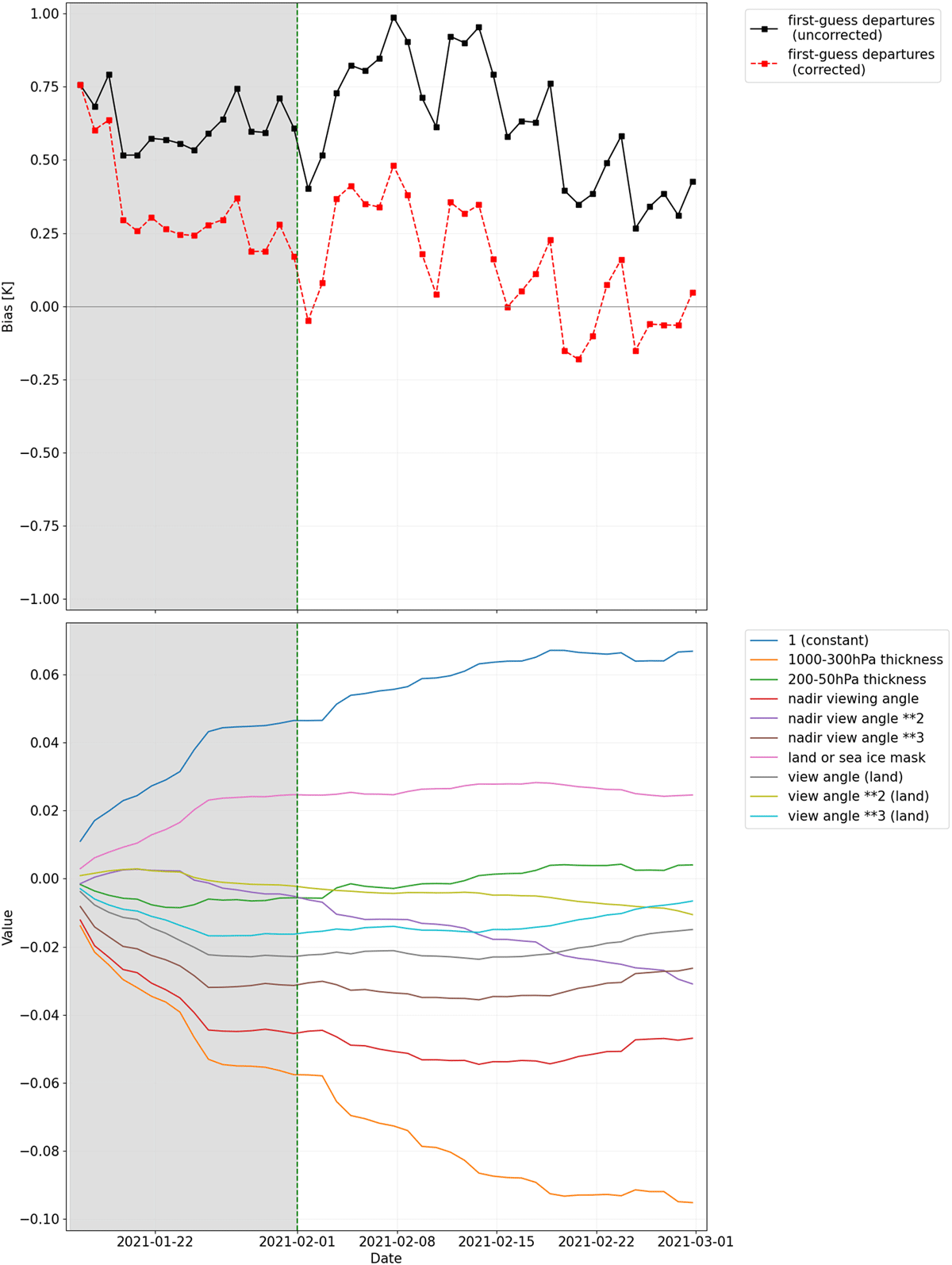
Figure 11
Time series of the “spin-up” process showing the evolution of uncorrected and corrected averaged First-guess departures (upper plot) and the 10 predictor values (lower plot) for AMSU-A channel 5. Values are extracted from the ctl-3D-Var configuration during the spin-up period (gray shaded background) and from ldyn-3D-Var configuration afterwards. Data are for the period from 15 January to 28 February over the MetCoOp domain.
3.3 Understanding the changes in the amount of active observations (discussion)
Having an efficient bias correction in place together with a good description of the surface modelization is crucial to allow the assimilation of microwave low-peaking channels in HARMONIE-AROME; however, it is also important to understand how the dynamic emissivity method is behaving in the context of 3D-Var and 4D-Var experiments. The effect of having a better representation of the surface is expected to significantly change the amount of active observations. As mentioned in Section 2.1, an observation can be actively assimilated after having successfully passed a series of tests which include: thinning to respect a minimum distance between two observations and a quality check based on the First-guess departures.
Figure 12 quantifies the amount of active observations in both control configurations and the differences per assimilation cycle, over one day. The amount of active observation in ctl-4D-Var is twice as large as ctl-3D-Var, especially for higher-peaking channels. These differences in terms of active observations are purely related to the DA method since the statistics are computed for both control ctl-4D-Var and ctl-3D-Var in which the dynamic emissivity method is not used and the low-peaking channels are blocklisted. In the HARMONIE-AROME 4D-Var configuration used in this paper, more observations are entering the radiative transfer model during the assimilation window partly because the thinning is done in 10 time slots (instead of a single one). As a result, the amount of available (and potentially active) AMSU-A observations might increase from about 5 % (up to 200 %) in the ctl-4D-Var compared to ctl-3D-Var.
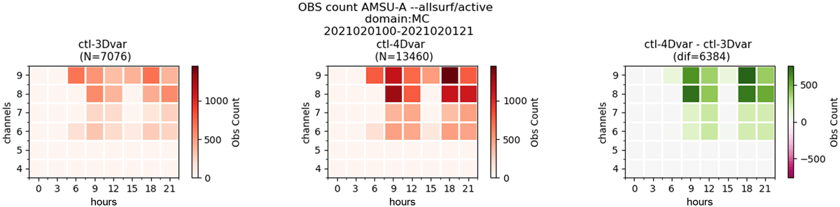
Figure 12
Count and differences of active radiance observations assimilated in both configurations ctl-3D-Var and ctl-4D-Var per AMSU-A channel and per assimilation cycle over the MetCoOp domain on the 1 February 2021.
Figure 13 shows histograms of First-guess departures over land at AMSU-A channel 4 (52.8 GHz) for a period of 5 days using different configurations. The figure illustrates the combined effect brought by the dynamic emissivity method and the data method used. In both systems, ctl-3D-Var and ctl-4D-Var, the dynamic emissivity method significantly improves the statistics in both terms of bias and standard deviation, leading to an increase of active observations too.
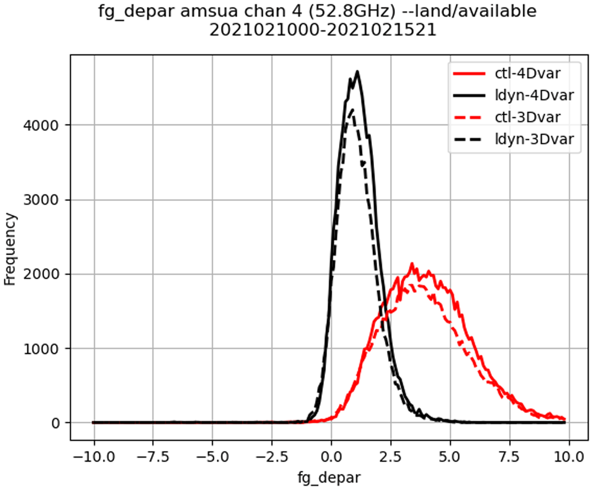
Figure 13
Frequency histograms of First-guess departures (not corrected from the VARBC) over land surface using all available observations (from 10 to 15 February 2021) at AMSU-A channel 4 for ctl-3D-Var, ctl-4D-Var and ldyn-3D-Var, ldyn-4D-Var over the MetCoOp domain.
To isolate the effect of the dynamic emissivity method, one can evaluate the changes in active data between experiments that use the same DA systems: i.e., ctl-3D-Var versus ldyn-3D-Var or ctl-4D-Var versus ldyn-4D-Var active data count. Figure 14 quantifies the amount of active AMSU-A and MHS observations per channel, per assimilation cycle, in both ctl-3D-Var and ldyn-3D-Var experiments and the difference between both configurations. As expected, the count for the higher-peaking channels (i.e., AMSU-A channels 8 and 9) is unchanged. AMSU-A channels 6 and 7, as well as MHS channels 3 and 4 counts are slightly increased. It could indicate that the information brought by the assimilation of channel 5 (together with the dynamic emissivity method) is propagated vertically to these channels that are peaking a bit higher in the atmosphere.
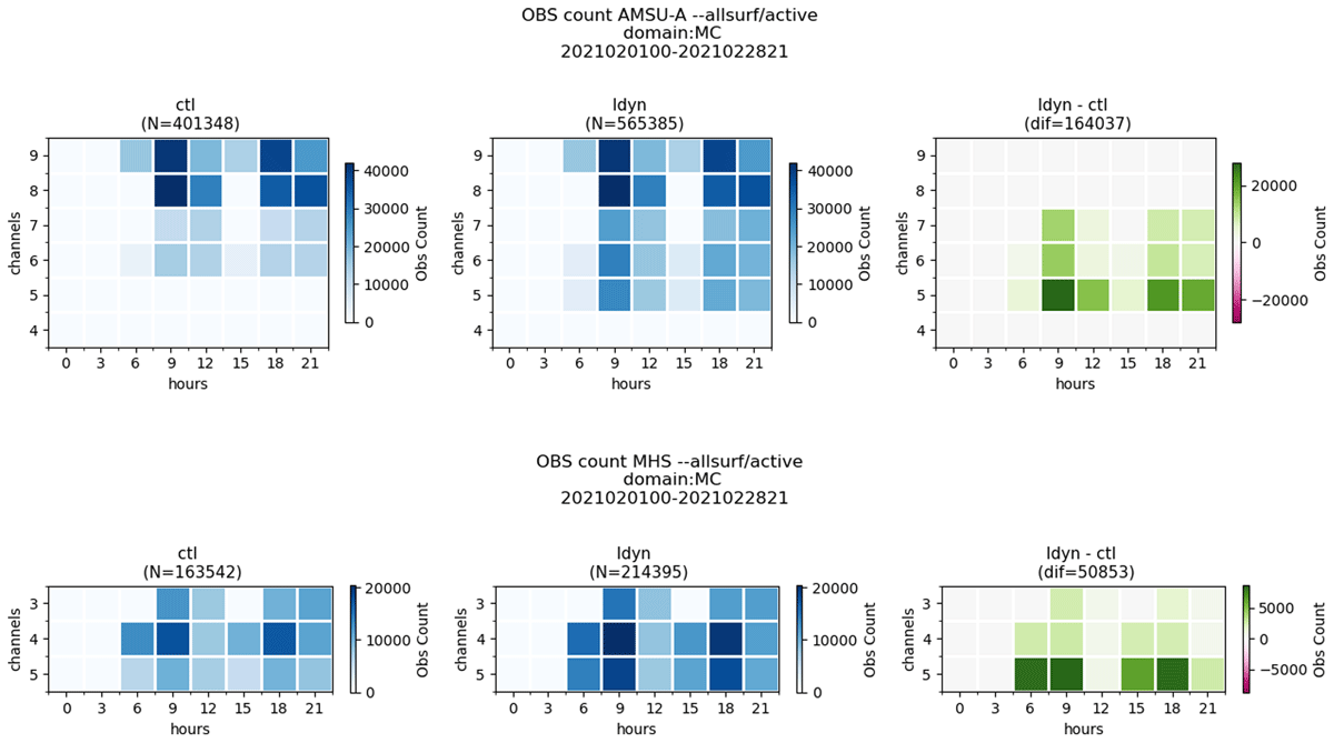
Figure 14
Count and differences of active radiance observations assimilated in both configurations ctl-3D-Var and ldyn-3D-Var per channel and per assimilation cycle over the MetCoOp domain on the period from 1 to 28 February 2021. Upper (lower) plots show the results for the AMSU-A (MHS) observations.
One could argue that, in return, via the cycling effect and for the specific case of the 4D-Var in which the observations are used at the correct time, the analysis can be considered better constrained (e.g., more observations are assimilated) and consequently, the quality of the next produced First-guess is also improved. Figure 15 shows the First-guess departure histograms for AMSU-A channel 5 over land surface and for three configurations: (1) ctl-4D-Var, which uses the default land surface emissivity as input, (2) nolwp-4D-Var, which uses the dynamic emissivity method but does not assimilate AMSU-A (neither MHS) channel 5; and (3) ldyn-4D-Var, which also uses the dynamic emissivity method and does assimilate both low-peaking channels. In fact, since ldyn-4D-Var describes the best statistics, it could be concluded that the active assimilation of AMSU-A channel 5 helps in reducing the First-guess departures, especially compared to the ctl-4D-Var control configuration.
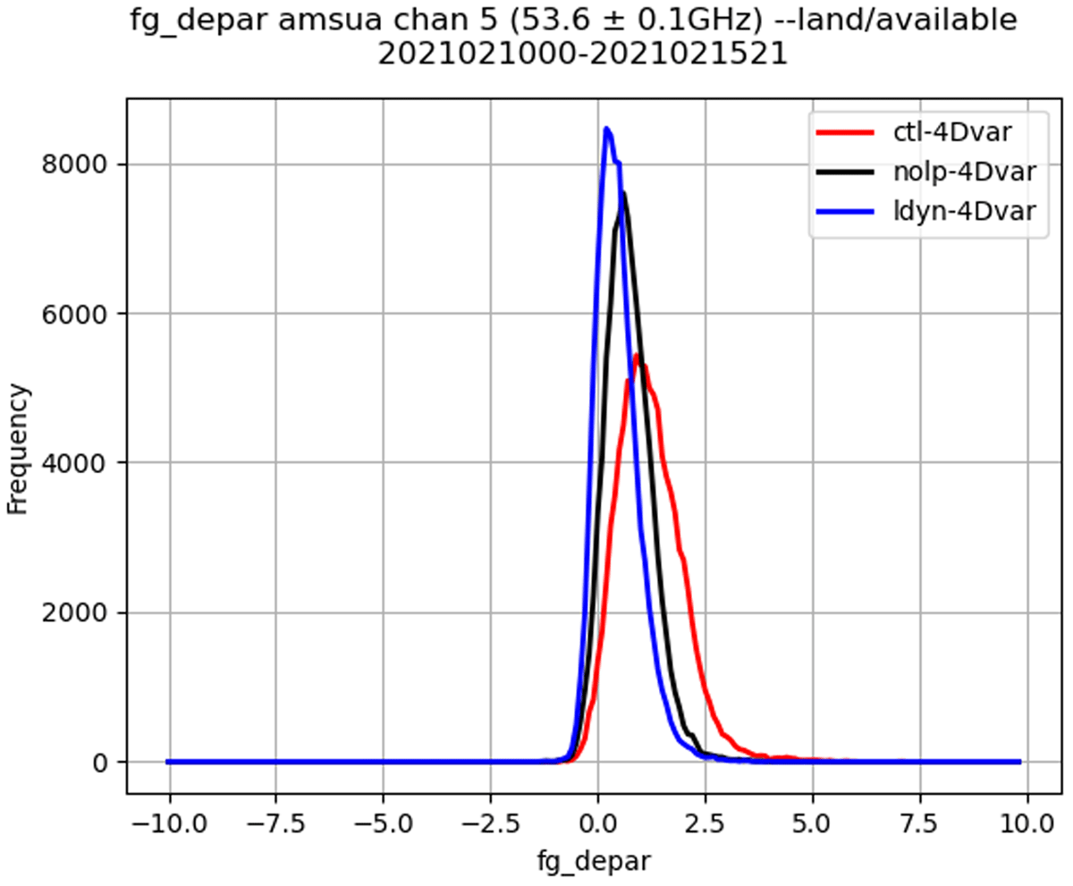
Figure 15
Frequency histograms of First-guess departures over land surface using all available observations (over 5 days from 10 to 15 February 2021) at AMSU-A channel 5 over the MetCoOp domain.
To go further into details regarding the impact of having more active AMSU-A and MHS low-peaking channels assimilated, the next subsection evaluates how the produced first guess fits the other observations.
3.4 Fit to observations
Studying the First-guess departures statistics by observation type is a frequently used method to evaluate the impact of changes in the DA system. The impact is evaluated using the ratio of normalized First-guess departures to observations between two experiments, with uncertainty estimates. If this ratio is smaller than 1, a reduction and hence an improvement in First-guess departures is observed, which means that the background from ldyn-4D-Var (or ldyn-3D-Var) is closer to the observation than the ctl-4D-Var (or ctl-3D-Var), respectively. Since observations remain unchanged, this improvement can only be attributed to a better background field. The uncertainty estimate is plotted as standard error bars. If the error estimate does not cross the vertical line at x = 1, statistical significance at the 95 % confidence level is achieved. The statistics are computed against temperature (T) or u- and v-wind components (U/V) from radiosondes (called TEMP T, TEMP U/V respectively) and aircraft (AIREP T, AIREP U/V) observations together with radiance data from the IASI hyperspectral sounder (e.g., long-wave temperature sensitive set of channels called IASI LW and Water Vapor sensitive channels called IASI WV).
Figure 16 shows the normalized differences in First-guess departures for a selection of observation types during the period from 1 to 28 February 2021 over the MetCoOp domain. The First-guess departures statistics in Figure 16 show the impact of assimilating low-peaking channels from AMSU-A and MHS in the 3D-Var and 4D-Var systems. Overall, the impact is neutral to positive, with significant improvements for MHS observations in both systems. Regarding the First-guess departures statistics for IASI in the 4D-Var system, outcomes show mixed results, and we have no well-founded explanation for this yet. Significant improvements can be observed for long-wave sensitive channels at 300 hPa and in water vapor sensitive channels at 450 hPa. In contrast to that, there are notable degradations in long-wave sensitive channels between 450 hPa and 600 hPa, along with water vapor sensitive channels around 250 hPa. For AMSU-A channels, the impact is predominantly neutral with a positive improvement observed at channel 6 in the 4D-Var system.
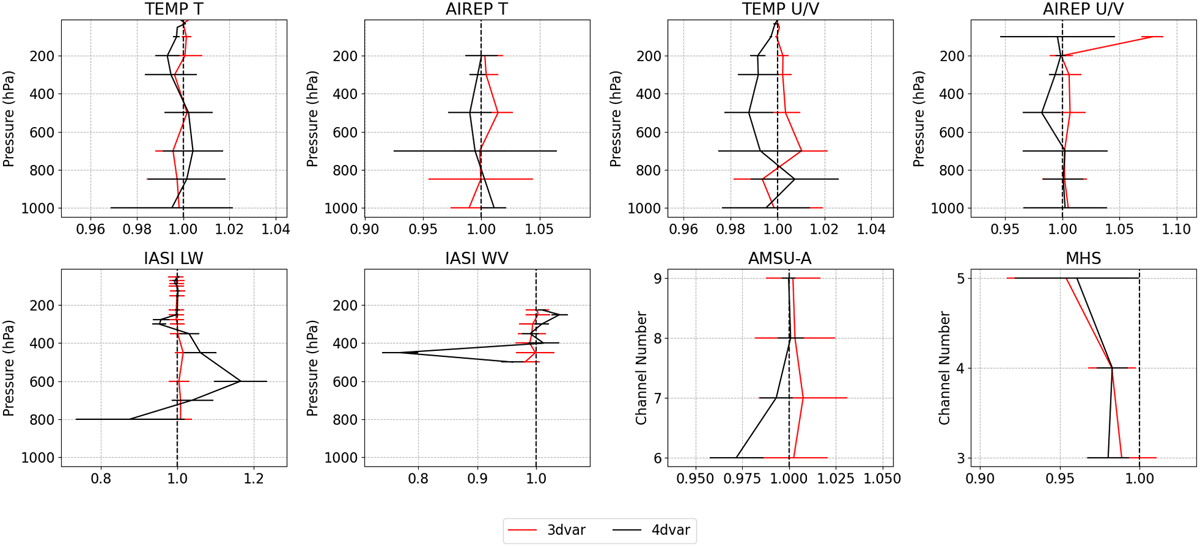
Figure 16
Normalized First-guess departures statistics of the 3D-Var (red) and 4D-Var (black) experiments of Temperature – Radiosonde (TEMP T) and Aircraft (AIREP T), u- and v-wind components – Radiosonde (TEMP U/V) and Aircraft (AIREP U/V), IASI long-wave sensitive (IASI LW) and IASI Water Vapor sensitive channels (IASI WV) by pressure levels and AMSU-A and MHS by channel number. For the period from 1 to 28 February 2021 over the MetCoOp domain.
3.5 Impact on the analysis and forecasts
In this section, analysis increments and forecast scores against conventional observations have been computed to evaluate the impact of low-peaking channels on the skills of the NWP system. The assimilation of low-peaking channel using the dynamical emissivity approach has a large impact on the analyses. This is most pronounced for atmospheric temperature and humidity at model levels in the lower troposphere, i.e., in the vicinity of the surface. Figure 17 shows the averaged analysis increments of humidity and temperature at model level 60 (around 140 m above ground) for ctl-3D-Var and ldyn-3D-Var runs. Substantial differences exist and are mainly attributed to land areas. With ldyn-3D-Var, there is a moistening of the lower atmosphere in large parts of the land areas. For temperature, the effect of dynamical emissivity is mainly confined to land areas as well, but not as clearly as for humidity. In addition, there is a warming attributed to ldyn-3D-Var in large areas of the Norwegian Sea. A similar effect of the dynamical emissivity method can be seen in 4D-Var humidity and temperature analyses (not shown). The results are consistent with results in the number of active observations, where the largest changes were found for low-peaking channels.
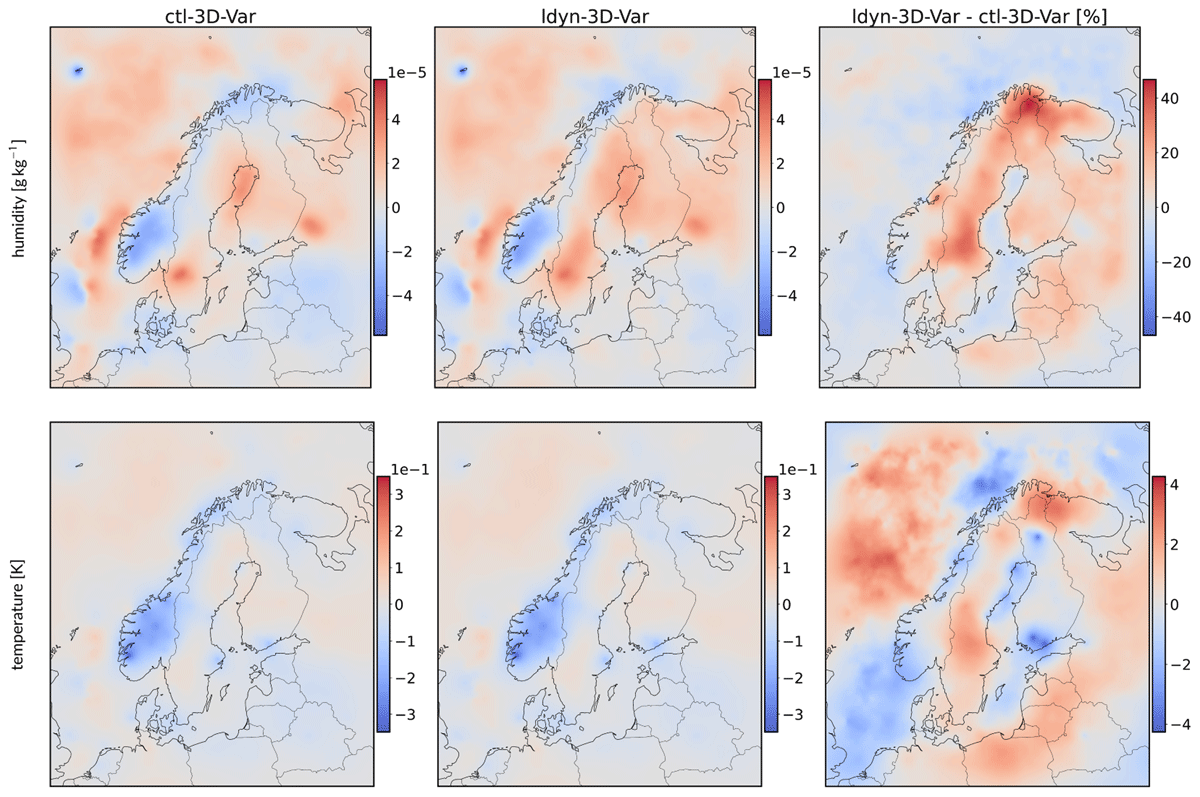
Figure 17
Averaged analysis increments of humidity (upper row, ) and temperature (lower row, ) at model level 60 for the 3D-Var system: ctl-3D-Var (left), ldyn-3D-Var (center), and the difference ldyn-3D-Var – ctl-3D-Var (right) in the period from 1 to 28 February 2021.
The moistening effect of the lower part of the atmosphere brought by the assimilation of low-peaking channels is in better agreement with the SYNOP measurements for relative humidity at 2 m (RH2m). This holds both when applied in 3D-Var and 4D-Var, as can been seen in Figure 18. The gentle warming effect of the dynamical emissivity method allows ldyn-4D-Var 2 m temperature (T2m) analyses, in terms of bias, to agree better with T2m observations compared to ctl-4D-Var. However, for 3D-Var, less agreement of ldyn-3D-Var T2m analyses with T2m SYNOP observations can be seen compared to ctl-3D-Var.
In Figure 18, the bias and normalized differences in the RMSE (Root Mean Square Error) are also shown for T2m and RH2m forecasts. For RH2m, improvements in bias and RMSE were obtained with 3D-Var and 4D-Var using the dynamical emissivity approach. The bias is reduced, and the normalized differences in RMSE are statistically significant. In terms of T2m, the most notable impact of the use of dynamical emissivity retrieval was on bias. The low-level warming effect by the use of dynamical emissivity resulted in increasing the initial-state bias for 3D-Var and reducing the bias in 4D-Var. This effect makes more biased 3D-Var forecasts, while 4D-Var is slightly improved, in terms of bias. When it comes to normalized differences in RMSE, a minor loss of skill is indicated for 3D-Var, although this is less than 1 % and only significant for a few early forecast lengths (approximately 3 h). Moreover, the normalized differences of RMSE indicate a consistent improvement in the forecast skill for all forecast ranges when applying the dynamical emissivity method in the 4D-Var setup. It is worth mentioning that improvements were obtained in the specific humidity, dew point temperature, and cloud cover forecast parameters, whereas for wind speed and MSLP (Mean Sea Level Pressure), the results are neutral (not shown here).
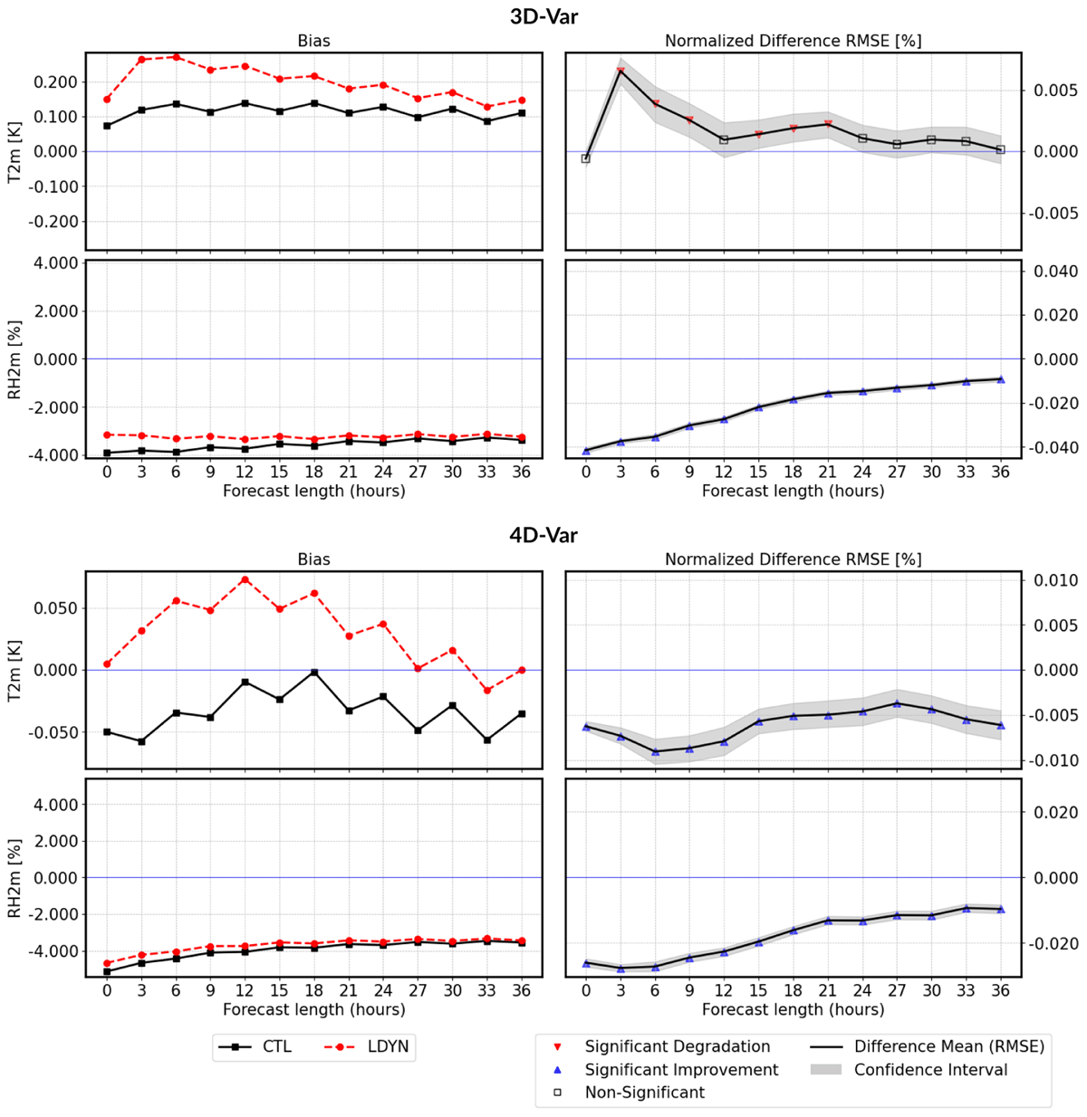
Figure 18
Bias and normalized RMSE (Root Mean Square Error) differences with uncertainty estimates of T2m and RH2m for the 3D-Var and 4D-Var experiments during 1–28 February 2021.
Verification of upper-air forecast variables like atmospheric temperatures, winds, and humidity against radiosonde measurements showed neutral results (not shown) for both 3D-Var and 4D-Var. Furthermore, due to the relatively small number of radiosonde observations compared to the number of SYNOP stations, the results were not statistically significant.
Scorecards provide a comprehensive overview of the forecast’s impact on a variety of variables that can be seen in Figure 19. As for the impact on RMSE, we see positive and often significant influences on the cloud variables cloud base height (Cbase) and total cloud cover (CCtot), as well as on the dew-point temperature (Td2m), 2 m humidity (Q2m), and RH2m variables. This positive impact was present for the first 24 hours of the forecast period. In contrast, the impact of the RMSE on surface pressure tends to be slightly negative but mainly insignificant. The impact on T2m appears to be negative in the case of 3D-Var, but positive in the case of 4D-Var. In general, there is a tendency that the dynamical emissivity approach has a larger positive impact within 4D-Var than using 3D-Var. One possible explanation for this is that 4D-Var is a more advanced DA scheme adapting better to improvements in observation handling. Another alternative complementing explanation is that, as shown before, more observations are used in 4D-Var than in 3D-Var. In the scorecard, it is evident that changes in forecast quality of the upper atmosphere, as verified against radiosonde observations, are small.
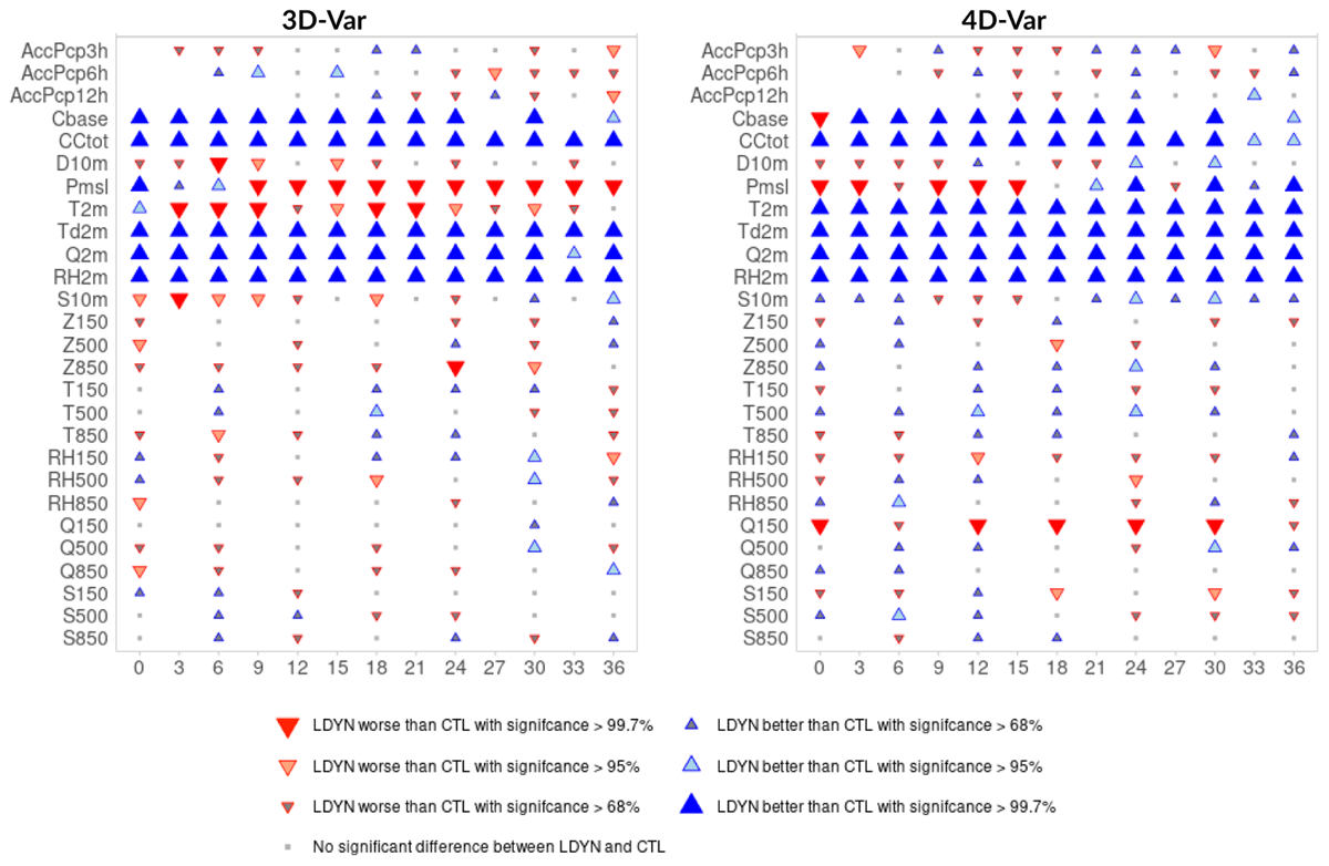
Figure 19
Scorecards of RMSE verification of surface and upper-Air variables for 3D-Var (left) and 4D-Var (right) experiments for period from 1 to 28 February 2021. Three sizes of blue upwards-facing triangles show levels of significant improvements of LDYN vs. CTL (99.7 % for the largest triangles, 95 % and 68 % for the smaller triangles). Vice versa for red downwards-facing triangles, which show degradations. See Appendix for the complete description of the variables.
4 Conclusion
This study is part of the preparatory work to use the innovative Arctic Weather Satellite (AWS) satellite being launched as a prototype for the recently approved constellation of small satellites (i.e., EPS-Sterna). An NWP configuration experiment has been built and run during the Calibration/Validation exercise of the AWS sounder. Also, this framework provided the opportunity to characterize and better understand the impact of operational microwave data on the HARMONIE-AROME regional model.
Focusing on the impact of assimilating AMSU-A and MHS microwave low-peaking channels with the dynamic emissivities, several experiments were run with both a 3D-Var and a 4D-Var DA system over the Nordic region. Positive impacts were obtained during a very cold winter period in 2021, which is an important achievement. In fact, the domain contains mostly snow- and ice-covered cold surfaces which induce, generally, the rejection of any low-peaking channel observations. Here, despite the sub-optimal use of the specular assumption to compute the surface emissivity over snow-covered surface, it was demonstrated that the dynamic emissivity is beneficial to assimilate more realistic surface-sensitive observations.
The improvements were consistent across various parts of the regional DA system, including the enhancement in number of active satellite microwave observations, suggesting a better fit between surface-sensitive channel observations and their First-guess equivalents, which in turn, may suggest an overall improvement in near-surface analyses and forecast fields. Significant improvements of the forecast skills were obtained against two-meter conventional observations of humidity for both 3D-Var and 4D-Var configurations, mostly up to 24 h forecast range. For two-meter temperature, the 4D-Var system seems to perform slightly better than 3D-Var with significant improvements despite a quantitative low impact (0.005 %).
The “so-called” dynamic emissivity method, as presented in (Karbou et al., 2010a), is still used nowadays in many global operational NWP systems (ECMWF, Météo-France among many others). In this paper, the benefit of this method has been explored at regional scale, in winter. It would be necessary to extend the study period for two reasons. First, one should consider increasing the spin-up duration for VarBC coefficients to a period twice longer than 15 days when using a cold start. Second, one should also consider running more tests over other seasons. In particular, these periods can involve snow/sea-ice melting, or intense storms. One should also consider retrieving the emissivity from a bias-corrected observation. For that, VarBC should be spun up for the window channels and the bias should be removed prior to the retrieval.
As it was mentioned earlier, this study was part of the successful ESA Performance Evaluation of Arctic Weather Satellite Data. Kicked off in 2021, this 4-year project set up the ground segment that enabled the reception and the processing of raw AWS data in real time. In parallel, a task was devoted to prepare the HARMONIE-AROME modeling system that permitted, recently, to run several On-the-fly DA experiments as part of the ESA Satellite In-Orbit Verification (SIOV) activities. First-guess departures to AWS radiance observations were produced for a few weeks, and regular useful feedback was given to ESA and industry. The instrument was declared operational following the Commissioning Results Review on 4 June 2025. At the time AWS was implemented to be ingested in HARMONIE-AROME, the assimilation of low-peaking channels was not considered over land and sea-ice. The dynamic emissivity method for AWS data has been recently implemented, and the operational monitoring of AWS radiances started officially on 26 November 2025, 09 UTC for AROME-Arctic, and it is expected to start in the coming weeks in the MetCoOp and United Weather Centres West (UWC-West) forecast systems.
Optimizing the impact of microwave sounding data has been an area of active research for many years. Here, the exploitation of low-peaking channels with the dynamic emissivity method has been studied. Following findings from Bormann et al. (2017), one should consider testing other surface hypotheses when retrieving the surface emissivity. In particular, promising results were obtained assuming the Lambertian approximation over snow-covered surfaces. These aspects are currently investigated further at SMHI and Met Norway. In addition, similarly to what has been done in Météo-France and ECMWF, one should also consider implementing the assimilation of AWS in all-sky conditions. The ESA/PRODEX Arctic Weather satellite All-sky Radiance data assimilation Implementation (AWARI) project, started at the Norwegian Meteorological Institute in May 2025, is taking over these activities to enable the optimal use of AWS (and EPS-Sterna) in the most challenging atmospheric and surface conditions (cloudy, rainy, snowy, sea-ice, snow-covered land, etc.).
Appendix: Scorecard variables
| CATEGORY | VARIABLE | DESCRIPTION |
|---|---|---|
| Accumulated | AccPcpXh | 3, 6, 12-hour accumulated precipitation |
| Precipitation | ||
| Clouds | Cbase | Cloud base height in metres |
| CCtot | Total cloud cover in oktas (eighths of the sky) | |
| Surface | Pmsl | Atmospheric pressure at mean sea level |
| Variables | T2m | 2-meter air temperature |
| Td2m | 2-meter dew point temperature | |
| Q2m | 2-meter specific humidity | |
| RH2m | 2-meter relative humidity | |
| S10m | 10-meter wind speed | |
| D10m | 10-meter wind direction | |
| Upper-air | Z | Geopotential height at 150, 500, 850 hPa |
| Variables | T | Air temperature at 150, 500, 850 hPa |
| RH | Relative humidity at 150, 500, 850 hPa | |
| Q | Specific humidity at 150, 500, 850 hPa | |
| S | Wind speed at 150, 500, 850 hPa |
Acknowledgements
The authors acknowledge Per Dahlgren for discussion on the specificity of the AWS instrument. We thank the anonymous reviewers for their constructive and detailed comments, which greatly contributed to improving the quality of this article.
Competing Interests
The authors have no competing interests to declare.