
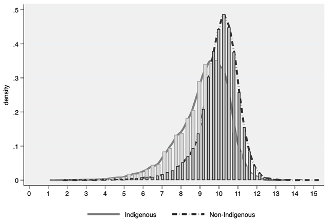
Figure 1
Distribution of the Logarithm of Monthly Wage by Ethnicity.
Source: Author’s calculations based on the ENIGH 2016.
Table 1
Descriptive Statistics by Ethnicity, 2016.
| Variable | Non-indigenous (n = 118,744) | Indigenous (n = 11,307) | ||
|---|---|---|---|---|
| Individual’s characteristics | Mean | Std. Dev | Mean | Std. Dev |
| Wage | 34,261 | 45,137.13 | 18,668 | 22,930.52 |
| Age | 38.41 | 14.64 | 41.54 | 16.21 |
| Years of schooling | 10.10 | 4.26 | 6.98 | 3.98 |
| Years of experience | 28.31 | 16.32 | 34.56 | 18.17 |
| Hours worked | 42.62 | 20.2 | 38.21 | 21.16 |
| Percentage | Percentage | |||
| Female | 39.77 | 39.09 | ||
| Locality Size | ||||
| Population of fewer than 2,500 | 35.53 | 64.78 | ||
| Between 2,500–14,999 inhabitants | 13.55 | 18.84 | ||
| Between 15,000–99,999 inhabitants | 13.45 | 7.81 | ||
| Population of more than 100,000 | 37.48 | 8.57 | ||
[i] Source: Author’s calculations based on the ENIGH 2016.
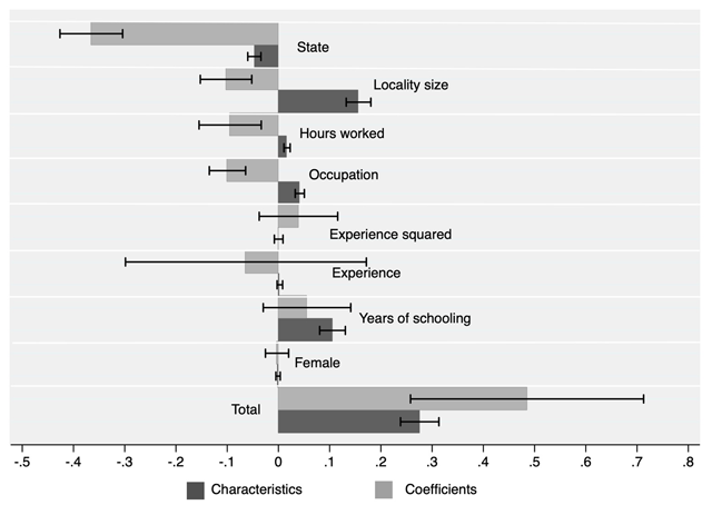
Figure 2
Two-fold Oaxaca-Blinder Wage Decomposition Results.
Notes: Indigenous is the reference category. Results show Heckman Correction estimates and bootstrapped standard errors with 50 replications.
Source: Author’s calculations based on the ENIGH 2016.
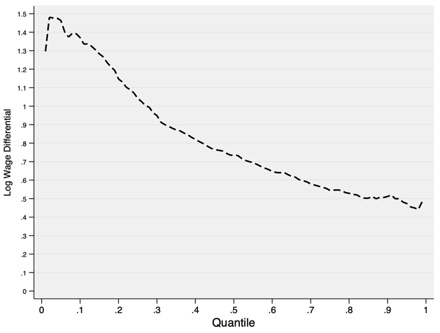
Figure 3
Mexico’s Raw Ethnic Wage Gap, 2016.
Source: Author’s calculations based on the ENIGH 2016.
Table 2
Conditional and unconditional quantile wage decomposition results.
| Quantile | θ= .10 | θ= .20 | θ= .30 | θ= .40 | θ= .50 | θ= .60 | θ= .70 | θ= .80 | θ= .90 |
|---|---|---|---|---|---|---|---|---|---|
| Raw Difference | –1.33*** | –1.13*** | –0.97*** | –0.85*** | –0.75*** | –0.67*** | –0.61*** | –0.54*** | –0.47*** |
| (0.02) | (0.02) | (0.02) | (0.01) | (0.01) | (0.01) | (0.01) | (0.01) | (0.02) | |
| Characteristics | –0.57*** | –0.49*** | –0.45*** | –0.43*** | –0.41*** | –0.40*** | –0.39*** | –0.38*** | –0.36*** |
| (0.01) | (0.01) | (0.01) | (0.01) | (0.01) | (0.01) | (0.01) | (0.01) | (0.01) | |
| Coefficients | –0.48*** | –0.46*** | –0.44*** | –0.42*** | –0.39*** | –0.36*** | –0.32*** | –0.28*** | –0.22*** |
| (0.02) | (0.02) | (0.02) | (0.01) | (0.01) | (0.01) | (0.01) | (0.02) | (0.02) | |
| Raw Difference | 1.41*** | 1.16*** | 0.96*** | 0.83*** | 0.72*** | 0.65*** | 0.58*** | 0.52*** | 0.50*** |
| (0.03) | (0.03) | (0.02) | (0.02) | (0.02) | (0.01) | (0.01) | (0.01) | (0.01) | |
| Characteristics | |||||||||
| Female | 0.00 | 0.00 | 0.00 | 0.00 | 0.00 | 0.00* | 0.00* | 0.00* | 0.00 |
| (0.00) | (0.00) | (0.00) | (0.00) | (0.00) | (0.00) | (0.00) | (0.00) | (0.00) | |
| Years of schooling | 0.07** | 0.09*** | 0.13*** | 0.14*** | 0.15*** | 0.15*** | 0.16*** | 0.17*** | 0.20*** |
| (0.03) | (0.02) | (0.02) | (0.02) | (0.01) | (0.01) | (0.01) | (0.01) | (0.02) | |
| Experience | –0.24*** | –0.20*** | –0.12*** | –0.07*** | –0.07*** | –0.03* | –0.02 | –0.02 | –0.02 |
| (0.04) | (0.03) | (0.02) | (0.02) | (0.02) | (0.01) | (0.01) | (0.01) | (0.01) | |
| Experience squared | 0.38*** | 0.29*** | 0.18*** | 0.11*** | 0.09*** | 0.05*** | 0.03* | 0.01 | 0.00 |
| (0.04) | (0.03) | (0.02) | (0.02) | (0.01) | (0.01) | (0.01) | (0.01) | (0.01) | |
| Occupation | 0.16*** | 0.18*** | 0.17*** | 0.14*** | 0.12*** | 0.12*** | 0.10*** | 0.07*** | 0.06*** |
| (0.01) | (0.01) | (0.01) | (0.01) | (0.01) | (0.01) | (0.01) | (0.01) | (0.01) | |
| Hours worked | 0.05*** | 0.06*** | 0.06*** | 0.05*** | 0.04*** | 0.04*** | 0.03*** | 0.03*** | 0.02*** |
| (0.01) | (0.01) | (0.01) | (0.00) | (0.00) | (0.00) | (0.00) | (0.00) | (0.00) | |
| Locality size | 0.21*** | 0.26*** | 0.28*** | 0.27*** | 0.24*** | 0.22*** | 0.23*** | 0.20*** | 0.19*** |
| (0.02) | (0.02) | (0.02) | (0.01) | (0.01) | (0.01) | (0.02) | (0.02) | (0.02) | |
| State | –0.10*** | –0.09*** | –0.11*** | –0.08*** | –0.07*** | –0.06*** | –0.05*** | –0.03*** | –0.02*** |
| (0.01) | (0.01) | (0.01) | (0.01) | (0.01) | (0.01) | (0.01) | (0.01) | (0.01) | |
| Coefficients | |||||||||
| Female | 0.03 | 0.01 | –0.02 | –0.02 | –0.02 | –0.03* | –0.03** | –0.04** | –0.03** |
| (0.03) | (0.02) | (0.02) | (0.01) | (0.01) | (0.01) | (0.01) | (0.01) | (0.01) | |
| Years of schooling | 0.05 | 0.05 | 0.01 | 0.03 | 0.04 | 0.07* | 0.09** | 0.11** | 0.16 |
| (0.07) | (0.05) | (0.04) | (0.03) | (0.03) | (0.03) | (0.03) | (0.03) | (0.04) | |
| Experience | –0.55** | –0.77*** | –0.51*** | –0.35*** | –0.33*** | –0.18** | –0.11 | –0.06 | 0.00 |
| (0.19) | (0.14) | (0.11) | (0.08) | (0.07) | (0.07) | (0.07) | (0.07) | (0.07) | |
| Experience squared | 0.19 | 0.50*** | 0.33*** | 0.22*** | 0.22*** | 0.14*** | 0.11** | 0.07* | 0.05 |
| (0.13) | (0.09) | (0.07) | (0.05) | (0.04) | (0.04) | (0.04) | (0.04) | (0.04) | |
| Occupation | –0.13*** | –0.22*** | –0.23*** | –0.18*** | –0.17*** | –0.17*** | –0.15*** | –0.11*** | –0.09*** |
| (0.03) | (0.02) | (0.02) | (0.02) | (0.01) | (0.01) | (0.01) | (0.01) | 0.02 | |
| Hours worked | 0.25*** | –0.12** | –0.17*** | –0.19*** | –0.16*** | –0.18*** | –0.15*** | –0.15*** | –0.07** |
| (0.06) | (0.05) | (0.04) | (0.03) | (0.03) | (0.03) | (0.03) | (0.03) | (0.03) | |
| Locality size | 0.00 | –0.18*** | –0.23*** | –0.25*** | –0.21*** | –0.20*** | –0.23*** | –0.20*** | –0.22*** |
| (0.04) | (0.03) | (0.03) | (0.02) | (0.02) | (0.02) | (0.03) | (0.03) | (0.03) | |
| State | –0.64*** | –0.60*** | –0.67*** | –0.52*** | –0.49*** | –0.40*** | –0.35*** | –0.28*** | –0.23*** |
| (0.06) | (0.05) | (0.04) | (0.03) | (0.03) | (0.03) | (0.03) | (0.03) | (0.03) | |
[i] Notes: N = 105,754; * p < 0.05, ** p < 0.01, *** p < 0.001; Bootstrap standard errors with 100 replications in parenthesis.
Source: Author’s calculations based on the ENIGH 2016.
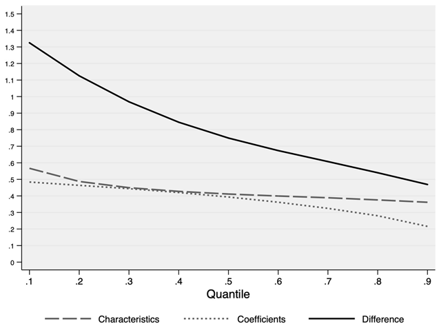
Figure 4
Quantile Decomposition of Mexico’s Ethnic Wage Gap, 2016.
Source: Author’s calculations based on the ENIGH 2016.
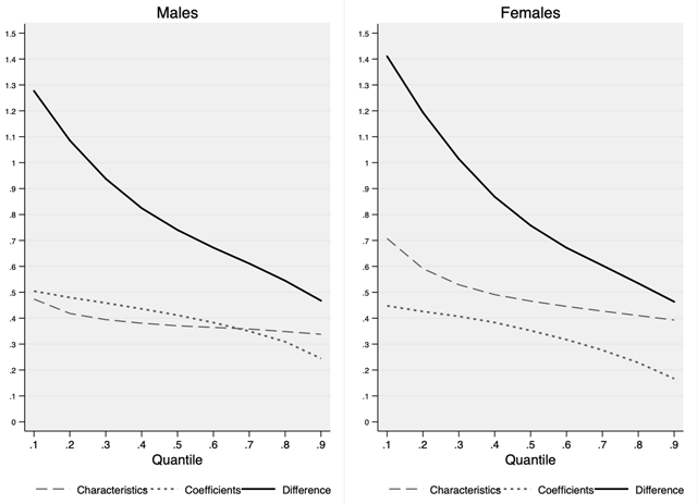
Figure 5
Quantile Decomposition of Mexico’s Ethnic Wage Gap by Gender, 2016.
Source: Author’s calculations based on the ENIGH 2016.
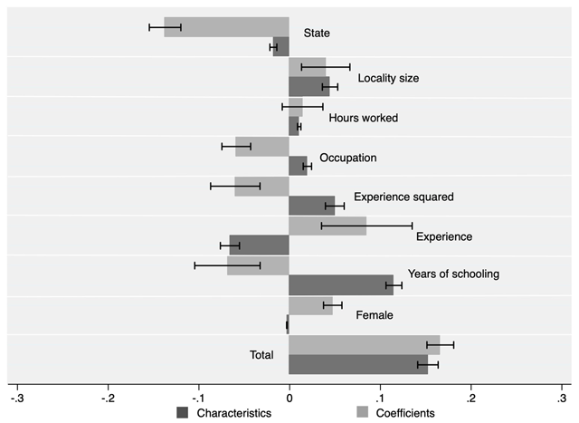
Figure 6
Decomposition Results of the Prevalence of Employment in the Informal Sector.
Source: Author’s calculations based on the ENIGH 2016.
Table 3
Decomposition Results of the Ethnic Gap in the Prevalence of Informal Employment by Gender.
| Total Sample | Females | Males | |
|---|---|---|---|
| Raw Difference | 0.32*** | 0.28*** | 0.37*** |
| (0.00) | (0.01) | (0.01) | |
| Characteristics | 0.15*** | 0.14*** | 0.19*** |
| (0.01) | (0.01) | (0.01) | |
| Coefficients | 0.17*** | 0.15*** | 0.18*** |
| (0.01) | (0.01) | (0.01) | |
| Characteristics | |||
| Female | 0.00*** | – | – |
| (0.00) | – | – | |
| Years of schooling | 0.11*** | 0.10*** | 0.14*** |
| (0.00) | (0.00) | (0.01) | |
| Experience | –0.07*** | –0.07*** | –0.08*** |
| (0.01) | (0.01) | (0.01) | |
| Experience squared | 0.05*** | 0.05*** | 0.08*** |
| (0.01) | (0.01) | (0.01) | |
| Occupation | 0.02*** | 0.03*** | 0.00 |
| (0.00) | (0.00) | (0.00) | |
| Hours worked | 0.01*** | 0.01*** | 0.02*** |
| (0.00) | (0.00) | (0.00) | |
| Locality size | 0.04*** | 0.06*** | 0.02** |
| (0.00) | (0.01) | (0.01) | |
| State | –0.02*** | –0.03*** | 0.00 |
| (0.00) | (0.00) | (0.00) | |
| Coefficients | |||
| Female | 0.05*** | – | – |
| (0.01) | – | – | |
| Years of schooling | –0.07*** | –0.06** | –0.12*** |
| (0.02) | (0.02) | (0.03) | |
| Experience | 0.09*** | 0.10** | 0.02 |
| (0.03) | (0.03) | (0.05) | |
| Experience squared | –0.06*** | –0.06*** | –0.02 |
| (0.01) | (0.02) | (0.03) | |
| Occupation | –0.06*** | –0.05*** | –0.04* |
| (0.01) | (0.01) | (0.02) | |
| Hours worked | 0.01 | 0.02 | –0.02 |
| (0.01) | (0.02) | (0.02) | |
| Locality size | 0.04*** | 0.01 | 0.11*** |
| (0.01) | (0.02) | (0.03) | |
| State | –0.14*** | –0.18*** | –0.04* |
| (0.01) | (0.01) | (0.02) | |
| N | 130051 | 78402 | 51649 |
[i] Notes: N = 76,001; * p < 0.05, ** p < 0.01, *** p < 0.001; Bootstrap standard errors with 100 replications in parenthesis.
Source: Author’s calculations based on the ENIGH 2016.
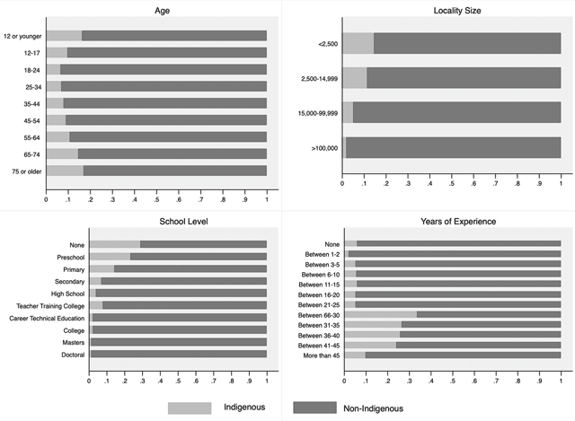
Figure A1
Structure of the Population by Socio-economic Characteristics.
Source: Author’s calculations based on the ENIGH 2016.
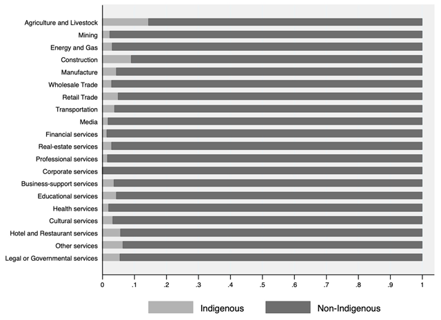
Figure A2
Structure of the Population by Occupational Sectors.
Source: Author’s calculations based on the ENIGH 2016.
Table A1
Two-fold Oaxaca-Blinder Wage Decomposition Results.
| Total Sample | Females | Males | ||||
|---|---|---|---|---|---|---|
| (1) | (2) | (1) | (2) | (1) | (2) | |
| Raw Difference | 0.83*** | 0.78*** | 0.85*** | 1.24*** | 0.81*** | 0.32 |
| (0.01) | (0.12) | (0.02) | (0.17) | (0.02) | (0.17) | |
| Characteristics | 0.51*** | 0.28*** | 0.57*** | 0.27*** | 0.46*** | 0.30*** |
| (0.02) | (0.02) | (0.03) | (0.03) | (0.02) | (0.03) | |
| Coefficients | 0.38*** | 0.49*** | 0.33*** | 0.91*** | 0.41*** | 0.04 |
| (0.01) | (0.12) | (0.02) | (0.17) | (0.02) | (0.17) | |
| Characteristics | ||||||
| Female | 0.00 | 0.00 | – | – | – | – |
| (0.00) | (0.00) | – | – | – | – | |
| Years of schooling | 0.14** | 0.11*** | 0.16*** | 0.11*** | 0.11*** | 0.11*** |
| (0.01) | (0.01) | (0.02) | (0.02) | (0.01) | (0.02) | |
| Experience | –0.11*** | 0.00 | –0.13*** | 0.01 | –0.10*** | 0.03* |
| (0.01) | (0.00) | (0.03) | (0.01) | (0.02) | (0.01) | |
| Experience squared | 0.15*** | 0.00 | 0.19*** | 0.02** | 0.13*** | –0.02** |
| (0.01) | (0.00) | (0.02) | (0.01) | (0.02) | (0.01) | |
| Occupation | 0.12*** | 0.04*** | 0.13*** | 0.02*** | 0.11*** | 0.04*** |
| (0.01) | (0.00) | (0.01) | (0.01) | (0.01) | (0.01) | |
| Hours worked | 0.04** | 0.02*** | 0.07*** | 0.03*** | 0.03*** | 0.02*** |
| (0.00) | (0.00) | (0.01) | (0.01) | (0.00) | (0.00) | |
| Locality size | 0.23*** | 0.16*** | 0.23*** | 0.14*** | 0.22*** | 0.16*** |
| (0.01) | (0.01) | (0.02) | (0.02) | (0.02) | (0.01) | |
| State | –0.06*** | –0.05*** | –0.08*** | –0.06*** | –0.05*** | –0.04*** |
| (0.01) | (0.01) | (0.01) | (0.01) | (0.01) | (0.01) | |
| Coefficients | ||||||
| Female | –0.01 | 0.00 | – | – | – | – |
| (0.01) | (0.01) | – | – | – | – | |
| Years of schooling | 0.08** | 0.06 | 0.06 | 0.08 | 0.09* | –0.01 |
| (0.03) | (0.04) | (0.04) | (0.06) | (0.04) | (0.06) | |
| Experience | –0.31*** | –0.06 | –0.26** | 0.37* | –0.33*** | –0.51* |
| (0.07) | (0.12) | (0.11) | (0.18) | (0.08) | (0.17) | |
| Experience squared | 0.17*** | 0.04 | 0.12 | –0.07 | 0.19*** | 0.09 |
| (0.04) | (0.04) | (0.06) | (0.07) | (0.05) | (0.05) | |
| Occupation | –0.14*** | –0.10*** | –0.18*** | –0.17*** | –0.12*** | –0.07*** |
| (0.01) | (0.02) | (0.02) | (0.04) | (0.01) | (0.02) | |
| Hours worked | –0.07** | –0.09** | –0.07* | –0.12** | –0.09* | –0.08 |
| (0.02) | (0.03) | (0.03) | (0.04) | (0.04) | (0.04) | |
| Locality size | –0.18*** | –0.10*** | –0.17*** | –0.05 | –0.19*** | –0.12*** |
| (0.02) | (0.03) | (0.04) | (0.05) | (0.03) | (0.03) | |
| State | –0.43*** | –0.37*** | –0.50*** | –0.44*** | –0.38*** | –0.32*** |
| (0.03) | (0.03) | (0.04) | (0.06) | (0.03) | (0.04) | |
| With Heckman Correction | N | Y | N | Y | N | Y |
| N | 105,754 | 101,168 | 43,639 | 41,552 | 62,115 | 59,616 |
[i] Notes: * p < 0.05, ** p < 0.01, *** p<0.001; Bootstrap standard errors with 100 replications in parenthesis.
Source: Author’s calculations based on the ENIGH 2016.