
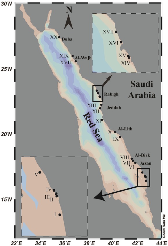
Figure 1
Map showing the study sites along the Saudi Arabian coast of the Red Sea
Table 1
Coordinates of different study sites along the Saudi Arabian coast of the Red Sea
| Location | Site No. | Latitude N | Longitude E | Remarks |
|---|---|---|---|---|
| Jazan | I | 16°25’6.85” | 42°45’49.08” | Fringing reef |
| II | 16°41’54.15” | 42°43’1.78” | Inland lagoon (dead mangrove) | |
| III | 16°43’54.71” | 42°42’29.12” | Inland lagoon (dead mangrove) | |
| IV | 16°47’3.69” | 42°40’23.07” | Fringing reef (near a sewage outlet) | |
| V | 17°3’3.16” | 42°27’8.85” | Fringing reef | |
| Al-Birk | VI | 17°48’0.89” | 41°53’21.16” | Inland lagoon (fish farm outlet) |
| VII | 17°57’9.17” | 41°41’10.91” | Fringing reef | |
| VIII | 18°7’11.42” | 41°34’52.77” | Fringing reef | |
| IX | 19°47’30.24” | 40°37’52.13” | Fringing reef | |
| Al-Lith | X | 20°9’56.94” | 40°12’50.01” | Inland lagoon (fish farm outlet) |
| Jeddah | XI | 21°16’8.74” | 39°7’34.40” | Fringing reef (sewage plant outlet) |
| XII | 21°58’57.73” | 38°58’44.60” | Inland lagoon | |
| XIII | 22°15’11.33” | 39°4’50.23” | Fringing reef | |
| Rabigh | XIV | 22°52’50.29” | 38°56’33.66” | Inland lagoon |
| XV | 22°51’3.09” | 38°57’35.99” | Inland lagoon | |
| XVI | 23°8’10.01” | 38°47’47.27” | Inland lagoon (fish farm outlet) | |
| XVII | 23°19’47.25” | 38°41’37.06” | Inland lagoon | |
| Al-Wajh | XVIII | 5°34’39.25” | 36°58’13.98” | Inland lagoon |
| XIX | 25°59’27.67” | 36°42’39.29” | Fringing reef | |
| Duba | XX | 27°25’52.30” | 35°36’9.54” | Inland lagoon |
Table 2
Differences in abiotic parameters of seawater (temperature – T and salinity – S) as well as sediment [pH, electrical conductivity – EC (mS cm−1); total organic carbon – TOC; and MD – mean grain size] observed at different sites along the Saudi Arabian coast of the Red Sea
| Site | Seawater | Sediment | ||||||
|---|---|---|---|---|---|---|---|---|
| T (°C) | S (PSU) | pH | EC (mS cm−1) | TOC (%) | MD (μm) | Sediment type | Sorting Index | |
| I | 28.9 | 38.56 | 8 | 6.9 | 3.5 | 353 | medium sand | poorly sorted |
| II | 28.5 | 43.1 | 8 | 5.3 | 3 | 296 | medium sand | poorly sorted |
| III | 31.1 | 40.3 | 7.05 | 22 | 3 | 356 | medium sand | poorly sorted |
| IV | 27.9 | 38.2 | 7.77 | 6.79 | 1 | 96 | very fine sand | moderately sorted |
| V | 28.9 | 40.1 | 7.6 | 10.26 | 3.7 | 208 | fine sand | poorly sorted |
| VI | 29.4 | 42.9 | 7.91 | 8.09 | 2.9 | 451 | medium sand | poorly sorted |
| VII | 28.7 | 41.5 | 6.75 | 9.95 | 3.3 | 243 | fine sand | poorly sorted |
| VIII | 28.5 | 39.3 | 7.45 | 10.1 | 2.5 | 229 | fine sand | poorly sorted |
| IX | 32.1 | 43.6 | 7.3 | 9.9 | 3 | 150 | fine sand | poorly sorted |
| X | 32.4 | 40.1 | 7.78 | 7.31 | 3.5 | 441 | medium sand | poorly sorted |
| XI | 29.3 | 43.1 | 7.82 | 10.1 | 1.8 | 156 | fine sand | poorly sorted |
| XII | 28.1 | 41.3 | 7.65 | 10.19 | 2.8 | 366 | medium sand | poorly sorted |
| XIII | 29.8 | 41.1 | 7.91 | 8.9 | 2 | 350 | medium sand | poorly sorted |
| XIV | 31.5 | 41.1 | 8.01 | 2.31 | 1.1 | 747 | coarse sand | moderately sorted |
| XV | 31.2 | 42.1 | 7.61 | 11.65 | 1.9 | 183 | fine sand | poorly sorted |
| XVI | 31.1 | 41.1 | 7.95 | 10.19 | 1.9 | 232 | fine sand | moderately sorted |
| XVII | 33.2 | 41.3 | 7.87 | 6.79 | 1.3 | 224 | fine sand | moderately sorted |
| XVIII | 36.2 | 42.1 | 7.91 | 6.49 | 1.7 | 197 | fine sand | poorly sorted |
| XIX | 35.1 | 43.5 | 7.85 | 6.8 | 1.6 | 249 | fine sand | poorly sorted |
| XX | 29.2 | 40.8 | 8.08 | 7.76 | 2.5 | 232 | fine sand | poorly sorted |
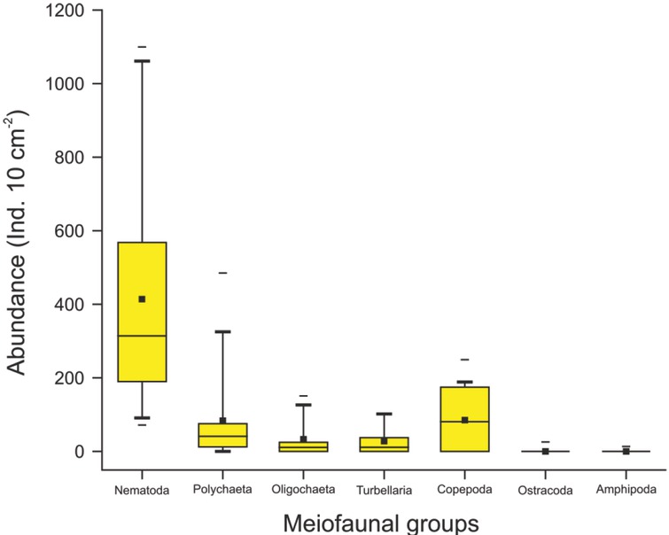
Figure 2
Box and whisker plot of different meiofaunal groups (ind. 10 cm−2) along the Saudi Arabian coast of the Red Sea. The bottom and the top of the boxes are the first and third quartiles, the band inside the boxes indicates the median, while the black square inside the box indicates the mean and the end of the whiskers expresses the range of abundance.
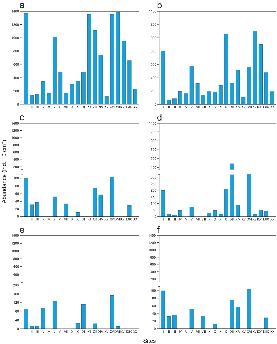
Figure 3
Spatial variations in abundance (ind. 10 cm−2) of: a) total meiofauna, b) nematodes, c) harpacticoid copepods, d) polychaetes, e) oligochaetes, and f) turbellarians observed at different sites along the Saudi Arabian coast of the Red Sea
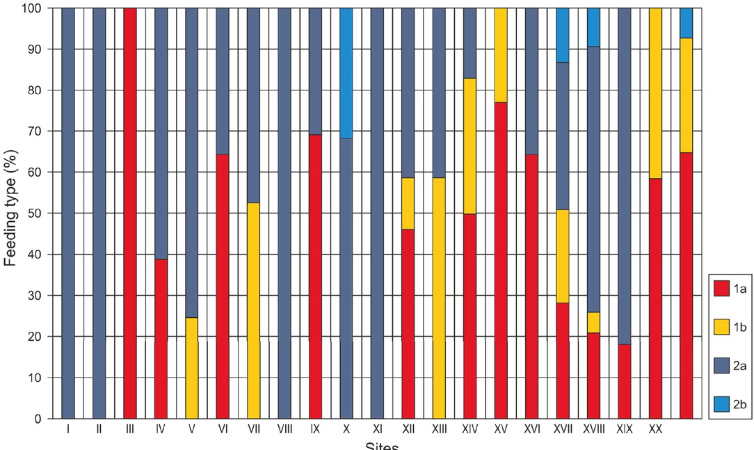
Figure 4
Relative abundance of each trophic status of nematodes at different study sites along the Saudi Arabian coast of the Red Sea. 1A – selective deposit feeders; 1B – non-selective deposit feeders; 2A – epigrowth feeders; 2B – predators/ omnivores
Table 3
Total count, relative abundance (%) and feeding types of different nematode genera recorded in mangrove sediments along the Saudi Arabian coast of the Red Sea. 1A – selective deposit feeders; 1B – non-selective deposit feeders; 2A – epigrowth feeders; 2B – predators/omnivores
| Order | Family | Genus | Total count | Relative abundance (%) | Feeding type |
|---|---|---|---|---|---|
| Enoplida | Ironidae | Syringolaimus | 1155 | 14.0 | 2a |
| Dolicholaimus | 86 | 1.0 | 2b | ||
| Oxystominidae | Halalaimus | 1336 | 16.2 | 1a | |
| Oncholaimidae | Viscosia | 85 | 1.0 | 2b | |
| Oncholaimus | 71 | 0.9 | 2b | ||
| Tripyloididae | Bathylaimus | 40 | 0.5 | 1b | |
| Aegialoalaimdae | Aegialoalaimus | 59 | 0.7 | 1a | |
| Chromadorida | Chromadoridae | Spilophorella | 91 | 1.1 | 2a |
| Metachromadora | 63 | 0.8 | 2a | ||
| Cyatholaimidae | Paralongicyatholaimus | 135 | 1.6 | 2a | |
| Selachinematidae | Synonochium | 49 | 0.6 | 2b | |
| Desmodoridae | Desmodora | 745 | 9.0 | 2a | |
| Molgolaimus | 29 | 0.4 | 2a | ||
| Spirina | 447 | 5.4 | 2a | ||
| Leptolaimidae | Leptolaimus | 48 | 0.6 | 1a | |
| Microlaimidae | Microlaimus | 1442 | 17.4 | 2a | |
| Bolbolaimus | 198 | 2.4 | 2a | ||
| Desmoscolecidae | Desmosolozenia | 17 | 0.2 | 1a | |
| Haliplectidae | Haliplectus | 63 | 0.8 | 1a | |
| Monhysterida | Xyalidae | Stylotheristus | 49 | 0.6 | 1b |
| Theristus | 196 | 2.4 | 1a | ||
| Paramonhystrea | 201 | 2.4 | 1b | ||
| Daptonema | 722 | 8.7 | 1b | ||
| Linhomoeidae | Metalinhomoeus | 90 | 1.1 | 1b | |
| Terschellingia | 849 | 10.3 | 1a |
Table 4
Values of Pearson’s coefficient of correlation (r) indicating possible relationships between meiofaunal groups and different environmental parameters (Meio – total meiofauna; Nema – nematodes; Poly – polychaetes; Oligo – oligochaetes; Turb – turbellarians; Cope – copepods; Ostr – ostracods and Amph – amphipods)
| Parameter | Meio | Nema | Poly | Oligo | Turb | Cope | Ostr | Amph |
|---|---|---|---|---|---|---|---|---|
| Sand (%) | 0.675** | 0.591** | 0.39 | 0.29 | 0.34 | 0.614** | 0.24 | 0.06 |
| VC sand | −0.13 | −0.11 | 0.03 | −0.30 | 0.13 | −0.22 | −0.26 | 0.12 |
| CS sand | 0.32 | 0.24 | 0.26 | 0.00 | 0.39 | 0.37 | −0.10 | 0.10 |
| M sand | −0.08 | −0.08 | −0.08 | −0.09 | −0.10 | 0.06 | 0.07 | 0.01 |
| F sand | 0.38 | 0.34 | 0.09 | 0.40 | 0.13 | 0.38 | 0.492* | −0.17 |
| VF sand | −0.448* | −0.35 | −0.23 | −0.09 | −0.502* | −0.573** | −0.28 | 0.01 |
| Silt-clay | −0.675** | −0.591** | −0.39 | −0.29 | −0.34 | −0.614** | −0.24 | −0.06 |
| pH | 0.39 | 0.33 | 0.31 | 0.32 | 0.35 | 0.12 | 0.16 | 0.13 |
| EC | −0.28 | −0.29 | −0.11 | −0.06 | −0.01 | −0.25 | 0.02 | −0.03 |
| OC (%) | −0.38 | −0.39 | −0.19 | −0.19 | −0.01 | −0.23 | −0.13 | −0.11 |
| Temperature | 0.17 | 0.31 | −0.10 | −0.25 | −0.09 | 0.08 | 0.06 | −0.08 |
| Salinity | −0.02 | 0.03 | −0.13 | −0.11 | −0.21 | 0.10 | −0.02 | −0.02 |
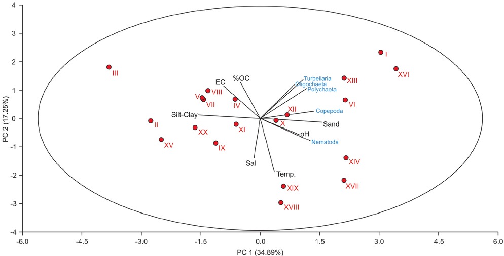
Figure 5
Principal component analysis (PCA) of normalized environmental variables and meiofaunal groups showing the main environmental gradient and relations along the surveyed sites
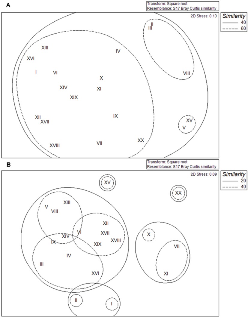
Figure 6
Multidimensional scaling (MDS) ordination based on the Bray-Curtis similarity indices of: A) different meiofaunal groups and B) nematodes
Table 5
Biodiversity indices of nematodes determined for different sites along the Saudi Arabian coast of the Red Sea: the total number of genera (S), richness (D), Pielou’s evenness index (J’) and Shannon-Wiener index (H’)
| Site | S | d | J’ | H’ (log) |
|---|---|---|---|---|
| I | 2 | 0.27 | 0.95 | 0.66 |
| II | 1 | 0.00 | 0.00 | 0.00 |
| III | 1 | 0.00 | 0.00 | 0.00 |
| IV | 3 | 0.63 | 1.00 | 1.10 |
| V | 2 | 0.35 | 0.95 | 0.66 |
| VI | 3 | 0.54 | 1.00 | 1.10 |
| VII | 3 | 0.59 | 0.99 | 1.09 |
| VIII | 1 | 0.00 | 0.00 | 0.00 |
| IX | 2 | 0.34 | 0.97 | 0.67 |
| X | 4 | 0.91 | 0.98 | 1.36 |
| XI | 2 | 0.32 | 0.97 | 0.68 |
| XII | 10 | 1.96 | 0.98 | 2.26 |
| XIII | 2 | 0.31 | 0.99 | 0.69 |
| XIV | 3 | 0.55 | 0.98 | 1.08 |
| XV | 2 | 0.37 | 0.94 | 0.65 |
| XVI | 4 | 0.80 | 0.91 | 1.26 |
| XVII | 11 | 2.15 | 0.98 | 2.36 |
| XVIII | 10 | 2.00 | 0.98 | 2.25 |
| XIX | 5 | 1.03 | 0.99 | 1.59 |
| XX | 2 | 0.34 | 0.99 | 0.69 |
Table 6
Meiofaunal abundance determined in different mangrove sediments worldwide (mean values given in parentheses)
| Area/Country | Densities (ind. 10 cm−2) | References |
|---|---|---|
| Minimum–Maximum (mean) | ||
| Hunter River, south-eastern Australia | 63–12057 (225) | Hodda & Nicholas (1985) |
| Hunter River, south-eastern Australia | 1–9596 (110) | Hodda & Nicholas (1986) |
| Northeastern Australia | 57–2454 | Alongi (1987a,b) |
| Mangrove mudflats, Australia* | 470–5000 (1830) | Nicholas et al. (1991) |
| Barwon estuary, Victoria, Australia | 250–8622 (2170) | Gwyther (2000) |
| Mngazana estuary, South Africa | 84–530 (246) | Dye (1983 a) |
| New Caledonia | 70–5137 | Della Patrona et al. (2016) |
| West and east coast of Zanzibar, Africa | 205–5263 (1493) | Ólafsson (1995) |
| West and east coast of Zanzibar, Africa | 271–656 | Ólafsson et al. (2000) |
| Gazi Bay, Kenya, Africa | 1986–6707 | Vanhove et al. (1992) |
| Island of Santa Catarina, South Brazil | 77–1589 (448) | Netto & Galucci (2003) |
| South Cuba | 36–245 | Lalana-Rueda & Gosselck (1980) |
| Gulf of Batabano, Cuba | 5–594 (109) | Armenteros et al. (2006) |
| West coast of Malaysia | 407–1109 (700) | Sasekumar (1994) |
| Southeast coast of India | 234–890 | Chinnadurai & Fernando (2007) |
| Northern Red Sea, Egypt | (343) | Pusceddu et al. (2014) |
| Sudanese coast of the Red Sea** | (288) | Sabeel (2015) |
| Western side of the Red Sea, Egypt | 18–193 (109) | El-Serehy et al. (2015) |
| Saudi Arabian coast of the Red Sea | 119–1380 (643) | Present study |
Table 7
Nematode abundance (mean in parenthesis), percentage of total meiofauna, richness and dominant genera recorded in different mangrove sediments worldwide
| References | Area/Country | Densities (ind. 10 cm−2) Minimum–Maximum (mean) | % of total meiofauna | Number of families | Number of genera |
|---|---|---|---|---|---|
| Hodda & Nicholas (1985) | Hunter River, south-eastern Australia | 63–11892 | 87–100 | 23 | 55 |
| Alongi (1987b) | Cape York, north-east Australia | 3–987 | – | (205 sp.) | |
| Nicholas et al. (1991)* | Mangrove mudflats, Australia | 113–451 | – | 26 | 38 |
| Dye (1983a) | Mngazana estuary, South Africa | 62–411 | 80.4 | – | – |
| Vanhove et al. (1992) | Gazi bay, Kenya | – | 54–95 | – | – |
| Ólafsson (1995) | West-east coast of Zanzibar, Africa | 131–5210 | 64-99 | 30 | 94 |
| Ólafsson et al. (2000) | West-east coast of Zanzibar, Africa | 271–656 | 58–87 | 13 | 28 |
| Netto & Galucci (2003) | Island of Santa Catarina, South Brazil | 196–811 | 85–94 | 28 | 86 |
| Pinto et al. (2013) | Pernambuco state, Northeastern Brazil | – | – | 25 | 73 |
| Armenteros et al. (2006) | Gulf of Batabano, Cuba | 5–591 (104) | 33–100 (88) | – | – |
| Ali et al. (1983) | Bay of Bengal, India | 35–280 | 50–67 | – | – |
| Chinnadurai & Fernando (2007) | Southeast coast of India | 234–890 | 86–93 | 20 | 36 |
| Bhadury et al. (2015) | Central west coast of India | – | – | 13 | 20 |
| Ansari & Bhadury (2017) | Sundarbans, India-Bangladesh | – | – | 29 | 84 |
| Somerfield et al. (1988) | North-western coast of Malaysia | (122) | – | 32 | 85 |
| Sasekumar (1994) | West coast of Malaysia | 374–885 | 80–93 | – | 17 |
| Sabeel (2015) | Sudanese coast, Red Sea | 10–370 | 40–98 | 20 | 35 |
| El-Serehy et al. (2015) | Western side of the Red Sea, Egypt | 8–162 (73) | 42(–6784) | – | – |
| Present study | Saudi Arabian coast of the Red Sea | 72–1100 | 29–100 | 15 | 25 |