
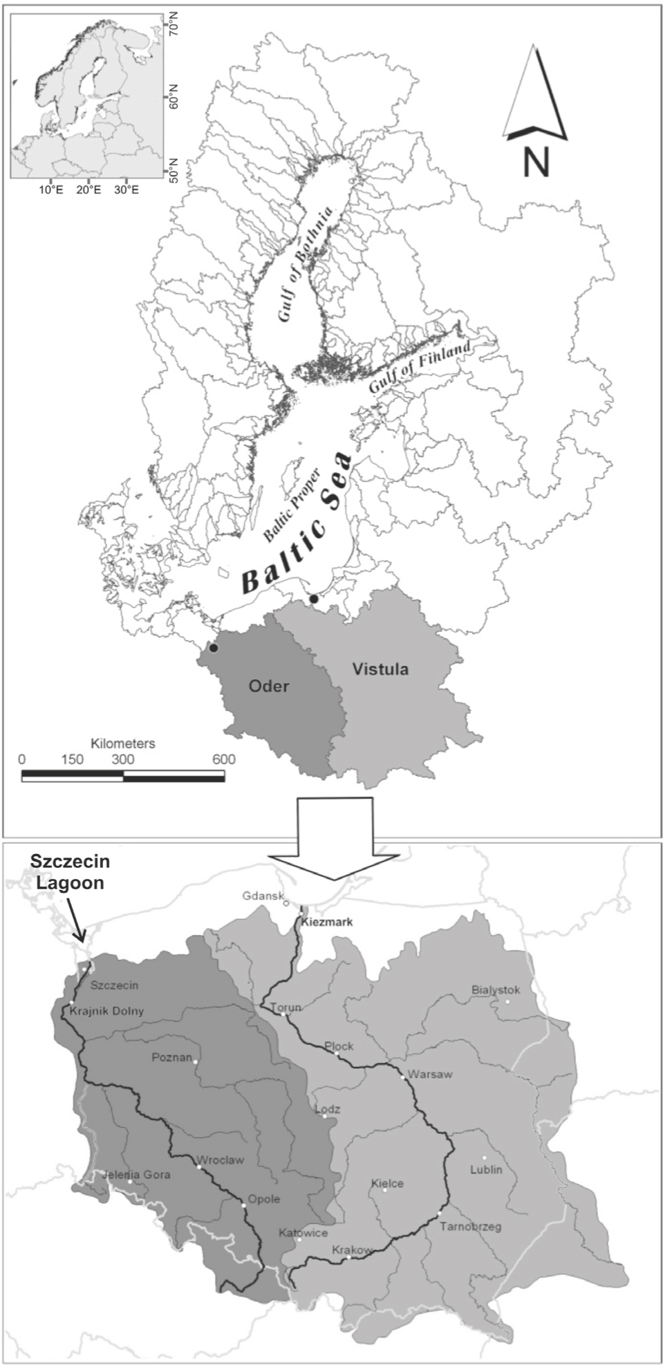
Figure 1
The Baltic Sea catchment and the location of the investigated Vistula and Oder basins; two dots in the upper map indicate the lowermost Oder (Krajnik Dolny) and Vistula (Kiezmark) monitoring stations (source: the upper part of the combined map was produced and kindly made available by Dr. Erik Smedberg from BNI, Stockholm University, Sweden)
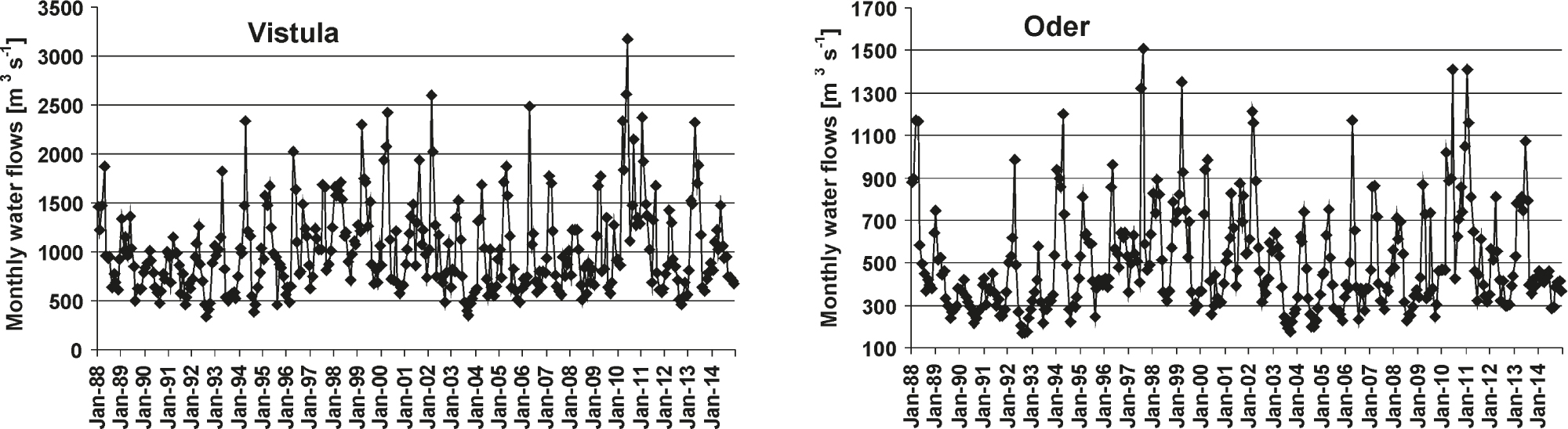
Figure 2
Average monthly water flows in the Vistula and Oder River in 1988–2014 (please note different scales)
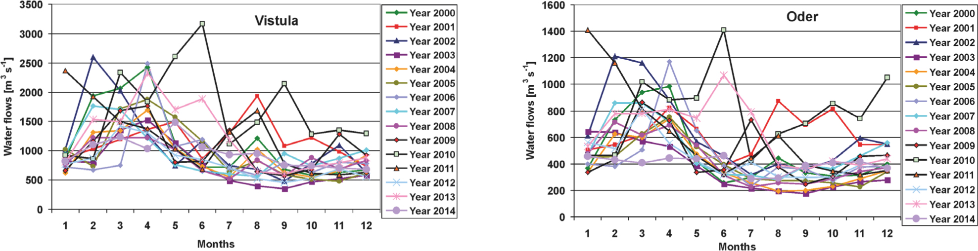
Figure 3
Seasonal variability of water flow in the Vistula and Oder River in 2000–2014 (please note different scales)
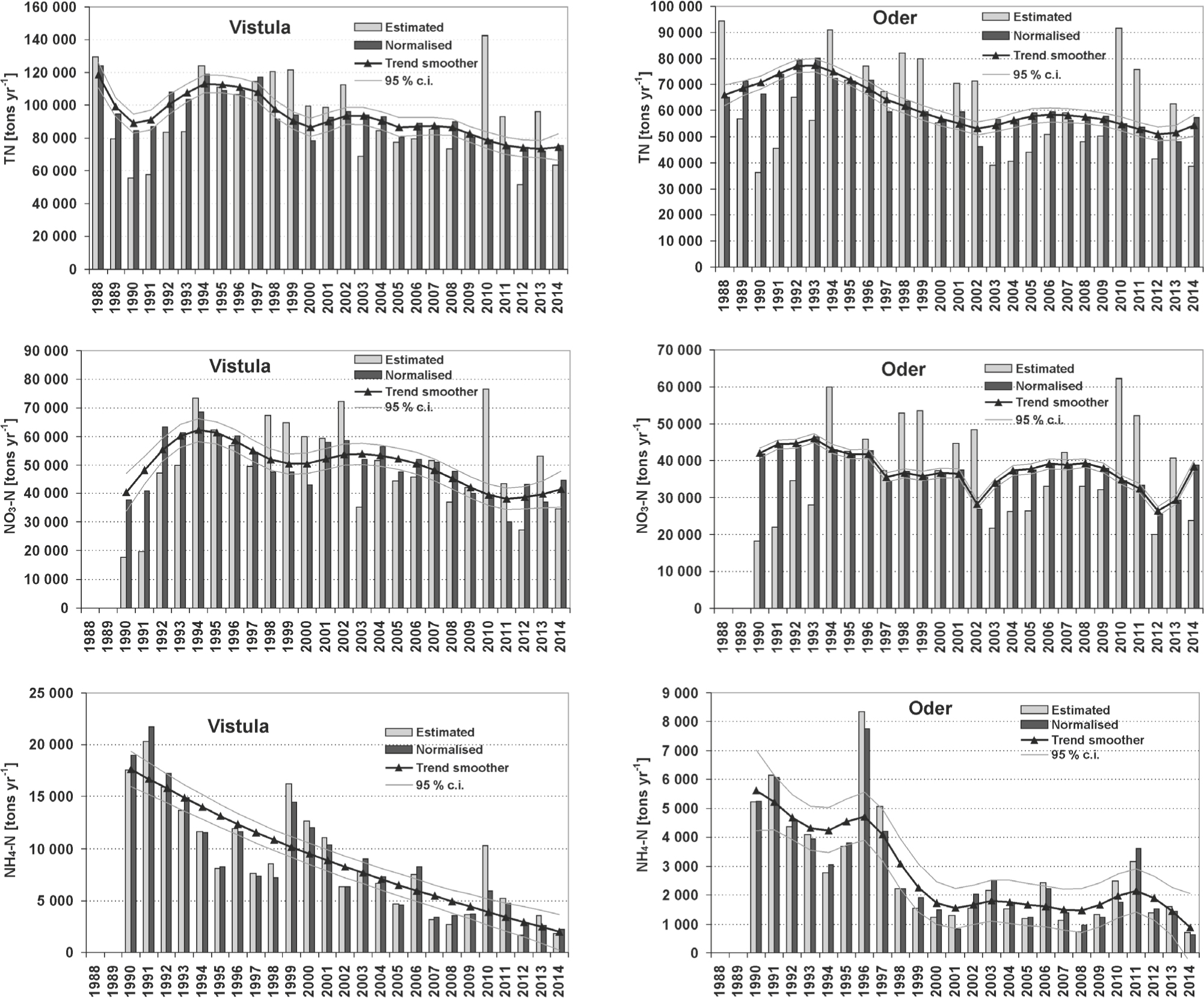
Figure 4
Estimated and flow normalized loads of nitrogen species at the lowermost river monitoring stations on the Vistula and Oder River in 1988–2014 (please note different scales)
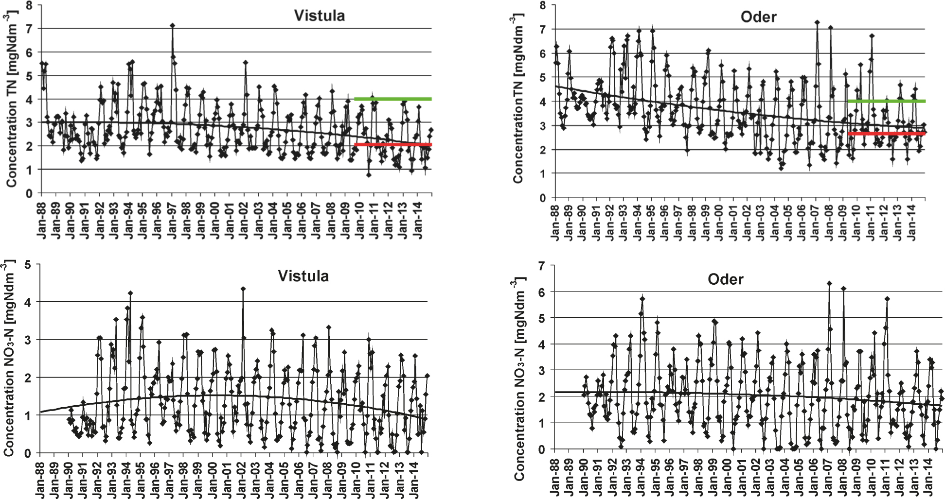
Figure 5
Concentrations of nitrogen species at the lowermost river monitoring stations on the Vistula and Oder River in 1988–2014;red lines in the TN graph indicate the calculated target concentrations with adopted HELCOM load reduction; green lines indicate target concentrations established for lowland large rivers (type 21; good ecological status acc. to the WFD) (see the Discussion; please note different scales)
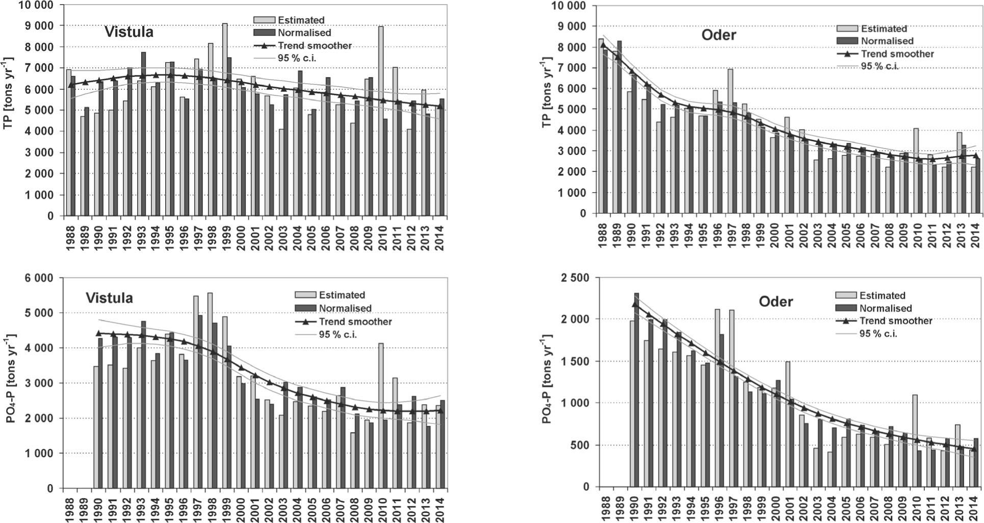
Figure 6
Estimated and flow normalized loads of phosphorus species at the lowermost river monitoring stations on the Vistula and Oder River in 1988–2014 (please note different scales)
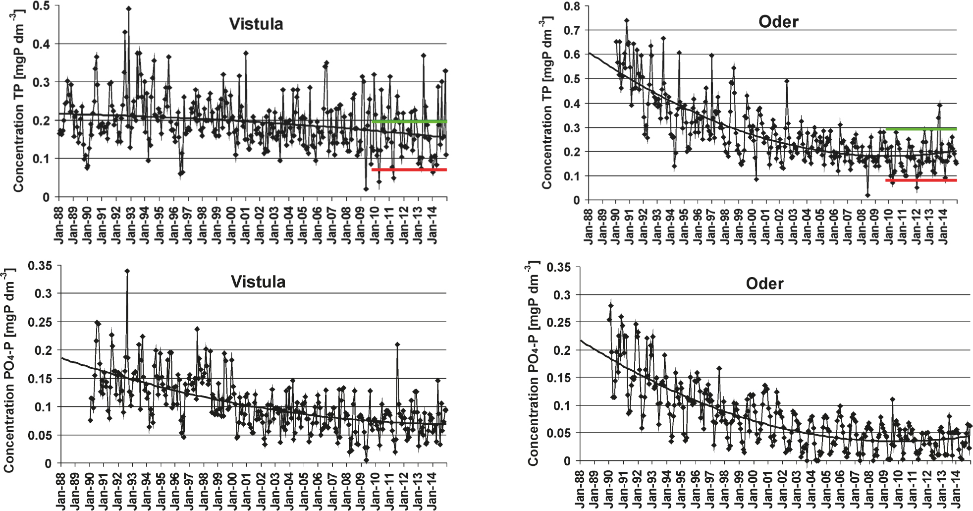
Figure 7
Concentrations of phosphorus species at the lowermost river monitoring stations on the Vistula and Oder River in 1988–2014; red lines in the TP graph indicate the calculated target concentrations with adopted HELCOM load reduction; green lines indicate target concentrations established for lowland large rivers (type 21; good ecological status acc. to the WFD) (see the Discussion; please note different scales)
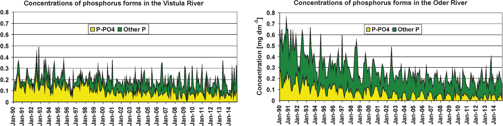
Figure 8
Concentrations of the phosphorus species at the lowermost river monitoring stations on the Vistula and Oder River in 1990–2014
Table 1
Country allocation of nutrient load reduction acc. to Country Allocated Reduction Target (CART) (HELCOM 2013a,b) and regional allocation of TP load reduction acc. to Håkanson et al. (2010)
| Country | HELCOM (2013a,b) approach | Håkanson et al. (2010) approach | |||||
|---|---|---|---|---|---|---|---|
| CARTTN [tons yr-1] | CART TP [tons yr-1] | Percentage contribution | Region | TP [tons yr-1] | TN [tons yr-1] | ||
| TN | TP | ||||||
| Denmark | 2890 | 38 | 3.24 | 0.26 | Bothnian Sea | Not needed | Reduction not recommended by the authors |
| Germany | 7670 | 170 | 8.59 | 1.18 | |||
| Poland | 43 610 | 7480 | 48.86 | 52.04 | Bothnian Bay | Not needed | |
| Lithuania | 8970 | 1470 | 10.05 | 10.23 | |||
| Latvia | 1670 | 220 | 1.87 | 1.53 | Gulf of Finland | 3180 | |
| Estonia | 1800 | 320 | 2.02 | 2.23 | |||
| Russia | 10 380 | 3790 | 11.63 | 26.36 | Gulf of Riga | 550 | |
| Finland | 3030 | 356 | 3.39 | 2.48 | |||
| Sweden | 9240 | 530 | 10.35 | 3.69 | Baltic Proper | 5000 | |
| Sum | 89 260 | 14 374 | 100.00 | 100.00 | 8730 | ||
Table 2
Combined flow normalized TN and TP loads discharged by the Vistula, the Oder, and the Pomeranian rivers in the reference period (1997–2003) and in 2012–2014, and the difference in loads in these two periods (yellow columns); maximum loads observed in 1992–1994 (TN) and 1988–1991 (TP), and the difference between maximum loads and those in 2012–2014 (green columns); allocation of load reduction acc. to BSAP (HELCOM 2013b) (red column)
| Nitrogen, phosphorus loads | In 1997–2003 | In 2012–2014 | Difference between 1997–2003 and 2012–2014 | Maximal observed (years in brackets) | Difference between max. observed and 2012–2014 | BSAP Poland |
|---|---|---|---|---|---|---|
| tons yr-1 | ||||||
| TN | 169648 | 140 372 | 29 276 | 209 243 (1992–1994) | 68 871 | 43 610 |
| TP | 11 548 | 8990 | 2558 | 14 903 (1988–1991) | 5913 | 7480 |
Table 3
Average combined flow normalized TN and TP loads, calculated for the reference period (1997–2003) for the Vistula and the Oder, and approximated for Polish rivers directly feeding the Baltic Sea, and target TN and TP concentrations at CART assumptions (Table 2); concentrations in brackets are offcially accepted maximum allowable values, meeting the good ecological status specified in WFD (Garcia et al. 2012)
| Average flow normalized TN loads | Average flow normalized TP loads | Target CART and max allowable WFD concentrations TN | Target CART and max allowable WFD concentrations TP | Target CART and max allowable WFD concentrations TN | Target CART and max allowable WFD concentrations TP |
|---|---|---|---|---|---|
| Vistula + Oder + other rivers | Vist | Oder | |||
| tons N yr-1 | tons P yr-1 | mg dm-3 | |||
| 94 794 + 57 220 + 17 634 = 169 648 | 6250+4116+1182= 11 548 | 2.06*) (4.00) | 0.067 (0.29) | 2.57*)(4.00) | 0.083 (0.29) |
such data are not available for our periods of calculations
Table 4
Eutrophication indicators in the brackish water systems (salinity 5–20 PSU) for four specified trophic states (source: Nixon 1995; Håkanson & Bryhn 2008)
| Trophic state | Håkanson and Bryhn (2008) | Nixon (1995) | ||||
|---|---|---|---|---|---|---|
| Secchi depth | Chl-a | TN | TP | Cyanobacteria | Organic carbon supply | |
| m | μg l-1 | μg wm l-1 | g C m-2 yr-1 | |||
| Oligotrophic | > 8 | < 2 | < 70 | < 10 | < 9.5 | < 100 |
| Mesotrophic | 4.5–8 | 2–6 | 70–220 | 10–30 | 9.5–380 | 100–300 |
| Eutrophic | 1.5–4.5 | 6–20 | 220–650 | 30–90 | 380–2500 | 301–500 |
| Hypertrophic | < 1.5 | > 20 | > 650 | > 90 | > 2500 | > 500 |
Table 5
Annual primary production [g C m-2 yr-1] in various regions of the Baltic Sea and various periods of time (source: Renk 2000 – publication of NMFRI)
| Area | Study period | |||
|---|---|---|---|---|
| 1971–1974 | 1981–1985 | 1987–1991 | 1994–1998 | |
| Gulf of Gdańsk (average value) | 140 | 156 | ||
| Gulf of Gdańsk (Gdansk Deep) | 107 | 129 | 172 | 190 |
| Bornholm Basin (Bornholm Deep) | 82 | 91 | 123 | 164 |
| Gotland Basin (Gotland Deep) | 92 | 116 | 141 | 140 |
| Słupsk Furrow | 88 | 103 | ||
Table 6
Average annual primary production [g C m−2 yr−1] in different regions of the Baltic Sea in 1954–2013 (source: Renk 2000 – publication of NMFRI; unpublished data of NMFRI)
| Area | Study period | Primary Production | Author(s) |
|---|---|---|---|
| Kattegat | 1954–1960 | 97.5 | Steemann Nielsen 1965 |
| 1964–1969 | 90.4 | Gargas et al. 1978 | |
| 1988–1990 | 290 | Richardson & Christoffersen 1991 | |
| Belt Sea | 1953–1957 | 86 | Steemann Nielsen 1965 |
| 1975–1977 | 116.5 | Gargas et al. 1978 | |
| Belt Sea – Sound | 1972 | 70–77 | Edler 1978 |
| 1973 | 73–183 | ||
| Belt Sea – Kiel Bight | 1971–1793 | 158 | Bodungen et al. 1975 |
| Bornholm Basin – Arkona Deep | 1971–1974 | 85 | Renk 1983 |
| 1967–1978 | 94.3 | Schulz & Kaiser 1973 and 1976 | |
| Bornholm Basin – Mecklenburg Bight | 1969–1978 | 130 | Kaiser et al. 1981 |
| Bornholm Basin – Bornholm Deep | 1967–1972 | 59–138 | Schulz & Kaiser 1974 and 1975 |
| 1971–1975 | 95 | Renk 1983 | |
| 1987–1991 | 123 | Renk 1997 | |
| Gulf of Gdansk | 1971–1974 | 140 | |
| 1987 | 304 | ||
| 2004–2013 | 138–285 | unpublished data, NMFRI | |
| average: 229 | |||
| Gulf of Gdańsk – Puck Bay | 1965–1991 | 198 | Renk 1997 |
| Gulf of Gdańsk – Gdansk Deep | 1971–1974 | 107 | |
| 1981–1985 | 129 | ||
| 1987–1991 | 172 | ||
| Gotlańd Basin – Gotlańd Deep | 1970 | 38 | Schulz & Kaiser 1973 |
| 1973 | 91 | Ackefors & Lindahl 1975 | |
| 1974 | 116 | Lindahl 1977 | |
| 1987–1991 | 141 | Renk 1991 and 1997 | |
| Aland Sea | 1974–1976 | 66–94 | Lindahl 1977 |
| Bothnian Bay | 1973–1974 | 18–70 | |
| Gulf of Finland | 1967–1971 | 30–65 | Niemi 1975; Bagge & Niemi 1971 |
| 78 | Forsskåhl et al. 1982 | ||
| Gulf of Finland – Helsinki area | 1968 | 150–200 | Bagge & Lehmusluoto 1971 |
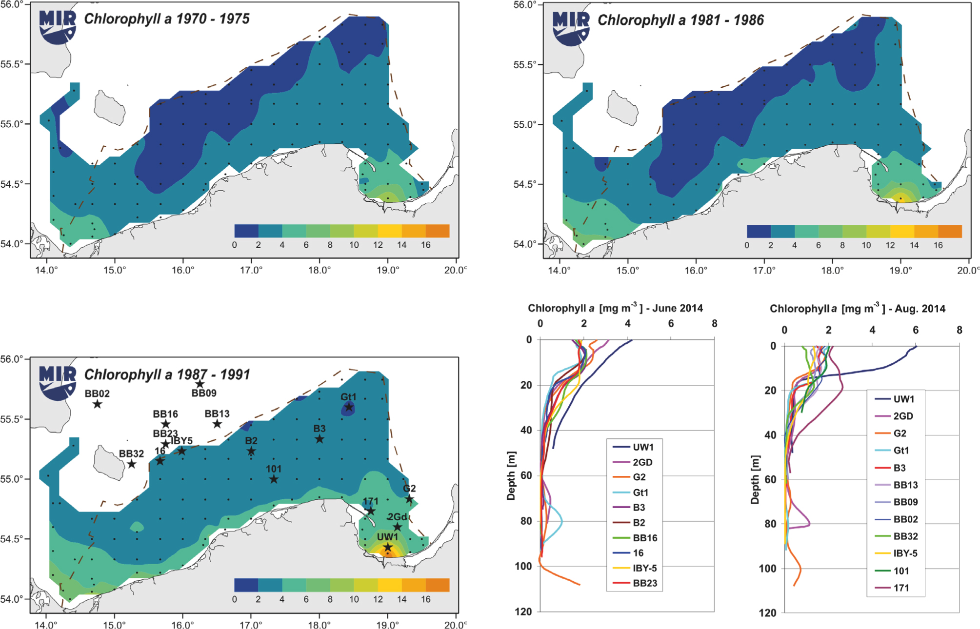
Figure 9
Average chlorophyll a concentrations (mg m-3) (mg m-3 = pg dm-3) in the summer season (July-September) in the 0–10 m layer in 1970–1975, 1981–1986, 1987–1991 (dots in the maps indicate sampled oceanographic stations) and vertical profiles of chlorophyll a concentrations (mg m-3) measured in June and August 2014 at oceanographic stations marked with asterisks (source: Renk 2000; Pastuszak et al. 2016; NMFRI data and publications)
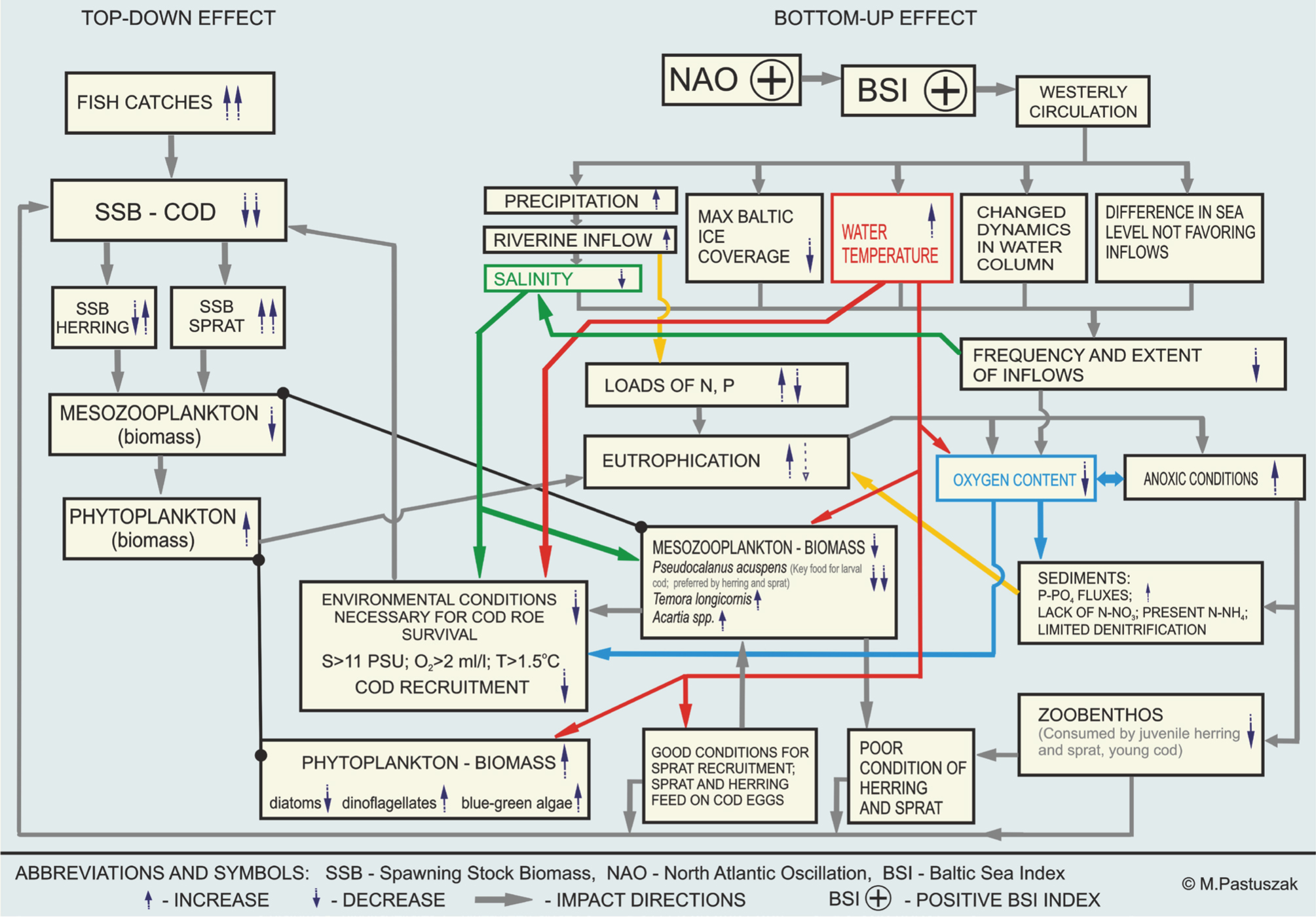
Figure 10
Top-down and bottom-up cascades and their interrelations in the Baltic Sea – biotic and abiotic parameters (source: graph was prepared based on the knowledge derived from the following publications: Alheit et al. 2004; 2005; Casini 2011; Casini et al. 2008; Cardinale & Arrhenius 2000; Cardinale et al. 2002; 2009; Conley et al. 2008; Dascalov 2002; 2011; Diekmann & Möllmann 2010; Flinkman et al. 1998; Håkanson et al. 2010; Hansson & Andersson 2015; Hare & Mantua 2000; Hinrichsen et al. 2002; Hurrell 1995; ICES 2011; Köster & Möllmann 2000; Köster et al. 2003; 2005; Lees et al. 2006; Mayer & Rietkerk 2004; Meier & Kauker 2003; Mohrholz et al. 2015; Möllmann 2011; Möllmann & Köster 1999; 2002; Möllmann et al. 2000; 2003; 2004; 2005; 2009; Overland et al. 2008; Rahm et al. 1996; Rönkkönen et al. 2004; Scheffer & Carpenter 2003; Schinke & Matthäus 1998; Scheffer et al. 2001; Wanner et al. 2001; Wasmund & Uhlig 2003)