
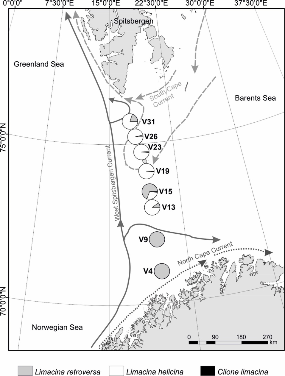
Figure 1
Map of species composition in the study area
Table 1
Sampling details with the specification of sampling stations
| Station | Longitude | Latitude | Sampling date | Time | Max haul depth (m) | Filtered water volume (m3) | Net obliquity (°) | Water mass |
|---|---|---|---|---|---|---|---|---|
| V31 | 75°42.002′N | 17°32.797′E | 10.08.2011 | 6:04:00 | 153 | 2128 | 50 | Atlantic |
| V26 | 74°57.001′N | 18°25.047′E | 10.08.2011 | 12:50:00 | 49 | 2115 | 45 | Arctic |
| V23 | 74°41.972′N | 18°39.208′E | 10.08.2011 | 15:30:00 | 57 | 1621 | 45 | Arctic |
| V19 | 74°09.897′N | 19°09.453′E | 10.08.2011 | 20:00:00 | 49 | 2381 | 45 | Arctic |
| V15 | 73°29.932′N | 19°19.694′E | 11.08.2011 | 1:00:00 | 212 | 4099 | 45 | Atlantic |
| V13 | 73°00.056′N | 19°27.466′E | 11.08.2011 | 6:10:00 | 212 | 4778 | 45 | Atlantic |
| V9 | 71°59.990′N | 19°41.012′E | 11.08.2011 | 15:00:00 | 141 | 3754 | 45 | Atlantic |
| V4 | 70°59.997′N | 19°53.924′E | 11.08.2011 | 20:00:00 | 106 | 4246 | 45 | Atlantic |
[i] *Net obliquity = line obliquity of the towing net
Table 2
Ranges of Limacina helicina, Limacina retroversa and Clione limacina densities (ind. 1000 m-3) at sampling stations
| Station | Limacina helicina | Limacina retroversa | Clione limacina |
|---|---|---|---|
| ind. 1000 m-3 | |||
| V31 | 177 | 44 | - |
| V26 | 12584 | 446 | - |
| V23 | 1317 | 26 | 15 |
| V19 | 1632 | 2 | 22 |
| V15 | 56 | 134 | 4 |
| V13 | 1213 | 136 | 1 |
| V9 | - | 1640 | 4 |
| V4 | 44 | 51826 | 267 |
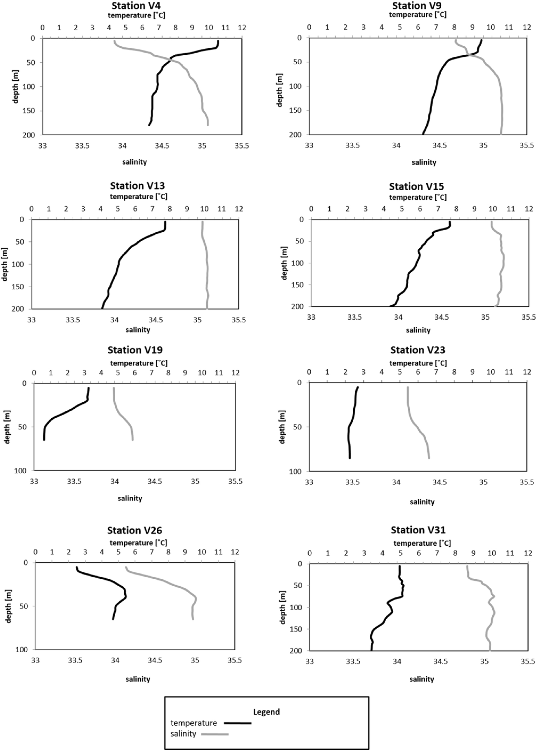
Figure 2
Variability in temperature and salinity of surface water at the sampling stations along the studied transect (the value of 200 m was used for the deeper stations and 100 m was used for the shallower stations)
Table 3
Chlorophyll concentration (mg m-3) in the study area
| Station | Chlorophyll (mg m-3) | |||||
|---|---|---|---|---|---|---|
| April | May | June | July | August | Mean | |
| V31 | 7.183 | 8.297 | 0.842 | 1.688 | 0.696 | 3.741 |
| V26 | 1.205 | 0.941 | 2.324 | 0.532 | 0.977 | 1.196 |
| V23 | 0.480 | 0.885 | 2.004 | 0.392 | 0.765 | 0.905 |
| V19 | 1.126 | 1.990 | 1.862 | NoData | 0.684 | 1.416 |
| V15 | 1.365 | 3.570 | 2.068 | 0.488 | 0.539 | 1.606 |
| V13 | 2.270 | 9.077 | 8.564 | NoData | 0.643 | 5.138 |
| V9 | 0.783 | 0.951 | 0.962 | 0.269 | 0.467 | 0.687 |
| V4 | 0.477 | 0.934 | 1.242 | 0.880 | 0.528 | 0.812 |
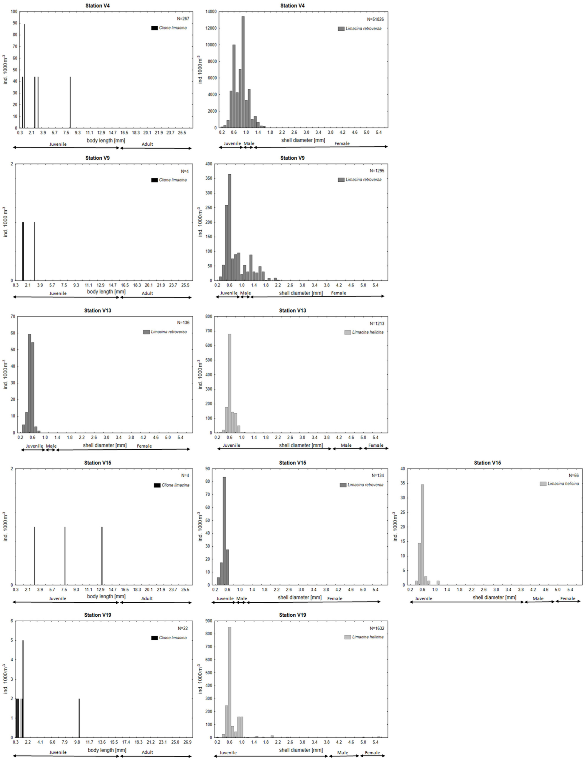
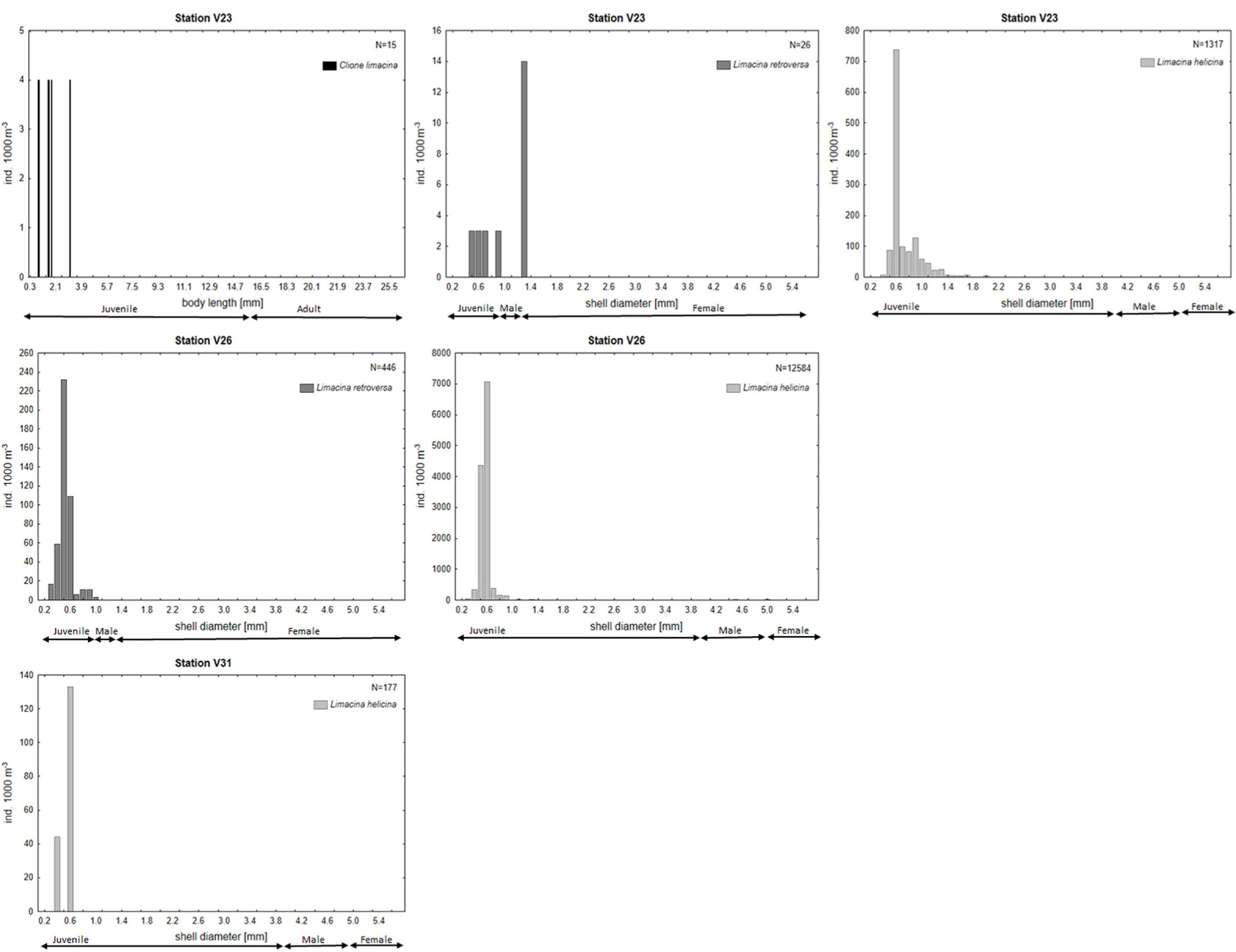
Figure 3
Size distributions for pteropods in the study area in August 2011 (some species were omitted due to the absence in the station area or due to the low abundance of specimens)
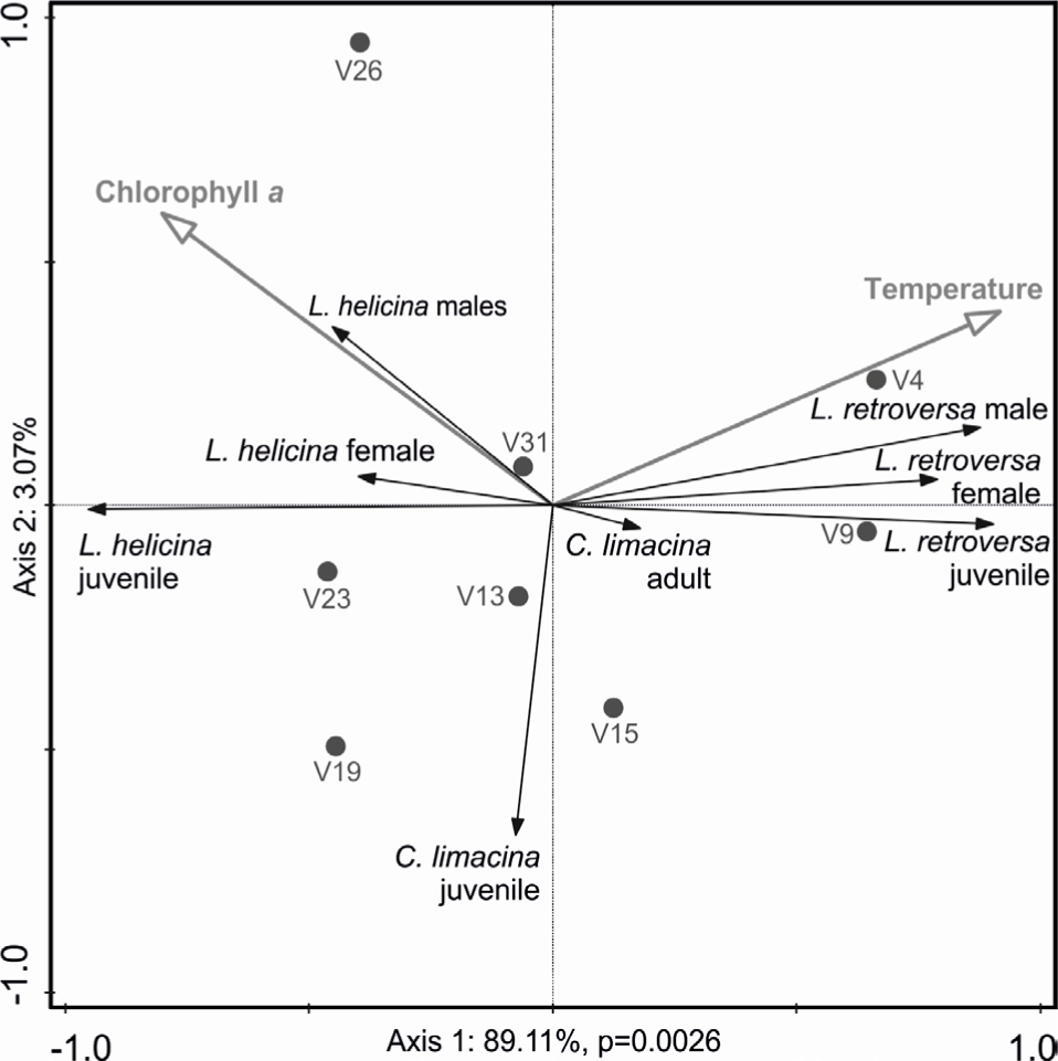
Figure 4
Redundancy analysis (RDA) ordination plot showing the relationship between the abundance of Pteropoda ontogenetic stages and the significant environmental variables, with the proportion of total variability explained by the first two canonical axes. Note that males and females are identified based on respective sizes.